26. The Zeeman Effect in Hydrogen and Alkali Atoms
Introduction
The Zeeman effect concerns the interaction of atomic systems with external magnetic fields. A basic understanding of the Zeeman effect is needed for many aspects of modern research in atomic physics. In addition, the Zeeman effect played an important historical role in the development of quantum mechanics, leading to the discovery of spin, the -factor of the electron, and the Thomas precession. In these notes we treat the Zeeman effect in one-electron atoms.
Units and Orders of Magnitude
We will use atomic units, so that . This means that , where is the fine structure constant. It also means that the Bohr magneton becomes
while the magnetic moment of the electron becomes
where we approximate for the electron factor. Thus, the energy of interaction of the electron spin in a magnetic field is
We must also deal with magnetic fields in atomic units. A magnetic field of strength in atomic units is equivalent to in ordinary Gaussian units, where is the unique magnetic field strength that can be constructed out of , and . That field is
where is the Bohr radius (the unit of distance in atomic units). is the strength of a magnetic field that is equal to the electrostatic field of the proton at the Bohr radius in the hydrogen atom (thus, it is also the atomic unit of electric field). Electric and magnetic fields have the same dimensions in Gaussian units, although one is usually called statvolts/cm and the other Gauss; see Appendix~\emunits. If an external field of strength is applied to a hydrogen atom in the ground state, the electron will feel a magnetic force that is of the order of times the electric force, since the velocity of the electron is . If you want to apply a magnetic field so strong that the magnetic force is equal to the Coulomb electric force from the nucleus, the field must have the strength . Such fields are so strong that atoms in the ordinary sense do not exist; the dynamics is dominated by magnetic forces at all distances larger than a Bohr radius. At higher magnetic field strengths, new physics appears. For example, at the strength , the energy of the lowest Landau level is becoming relativistic.
For reference, the strongest steady magnetic fields that can be created in a laboratory are of the order of 10~T or 105~Gauss. By using explosives or other means to compress magnetic flux, fields of the order of 103~T or 107~Gauss can be created for a short period of time. In astrophysics, much stronger magnetic fields arise. It is believed that at the surface of a neutron star there exist magnetic fields of up to 1012 Gauss, and there is speculation about fields of up to 1015 Gauss in “magnetars”. Because of these astrophysical applications, there has been some interest in recent years in the exotic physics that arises at high field strengths. In these notes we will assume that the external fields are steady state fields created in the laboratory, and hence have a maximum value of about 105~Gauss or 10-2 atomic units.
The Hamiltonian and Neglected Terms
In atomic units, the Hamiltonian for the electron in a single-electron atom (hydrogen-like or alkali) is
where the charge of the electron is , where is the central force potential (either Coulomb for hydrogen or screened Coulomb for alkalis), and where is the sum of the fine-structure corrections presented in (25). We assume a uniform magnetic field,
and we take the gauge
which is Coulomb gauge so that . This implies
so the cross terms in the expansion of the kinetic energy can be written in either order.
We expand the kinetic energy in the Hamiltonian (5) into three terms,
The cross term can also be written,
where . The third term can also be written,
It looks like a potential (it is a function only of the particle coordinates).
We estimate the relative order of magnitude of the three terms in the kinetic energy by first looking at the ratio,
where we use for a reference a state of hydrogen with quantum numbers that are of order unity, so that (the momentum of the electron in atomic units) and (its angular momentum) are both of order unity. Since we have decided that (in atomic units) is no more than 10-2, this ratio is about 10-4 maximum, and . Similarly, we find that the ratio is of the same order of magnitude, so is much smaller in turn than .
The term is of the same order of magnitude as the energy of interaction of the spin with the magnetic field (the last term in (5), and taken together these terms form what we shall call the Zeeman Hamiltonian,
The 2 multiplying the spin is really the -factor of the electron, indicating that different kinds of angular momentum produce magnetic moments in different proportions.
The Zeeman Hamiltonian is of the same order of magnitude as , which by our assumptions is at most about 10-4 in atomic units. This coincidentally is the same order of magnitude as the fine structure terms , at least in hydrogen, where they are of order . Of course by decreasing the strength of the magnetic field we can make . Similarly, by going to excited states, where fine structure effects are smaller than in the ground state, we can make . In the following we will analyze both limits in the comparison between and . As for the term , it is much smaller than any of the other terms, and we drop it. The result is the Hamiltonian that we will use for our analysis of the Zeeman effect,
where is given by (13).
Case I. Dominant, Negligible
The first case we shall consider is one in which is so much larger than that can be neglected altogether. This might require unrealistically large magnetic fields by laboratory standards (it depends on the quantum numbers), but it provides a useful reference for later work.
To analyze this case we take the unperturbed Hamiltonian and the perturbation to be
The unperturbed Hamiltonian is the nonrelativistic, electrostatic model of the atom, but we include the spin degrees of freedom in the wave functions. Thus, for hydrogen the energies are with degeneracies , and for the alkalis the energies are with degeneracies .
Thus we must think about degenerate perturbation theory. As usual, a good choice of basis of unperturbed eigenstates inside the degenerate, unperturbed eigenspaces may simplify the calculation (see \finestruc.5). The obvious choices of unperturbed eigenbases are the uncoupled basis, , and the coupled basis, . To see which is better, we make a table indicating which operators commutes with. We only list the -component of various angular momentum operators in the table, because the perturbation breaks the full rotational symmetry of the unperturbed system, and can only be invariant with respect to rotations about the -axis.
Table 1:The table indicates whether commutes with the given angular momentum operator (, ).
Y | Y | Y | Y | N |
|---|
We find that all the operators in the list commute with , except , which fails because contains the - and -components of and , which do not commute with or . The table makes it clear that the uncoupled basis is better for the perturbation calculation, since the operators of the complete set that define the uncoupled basis all commute with . Thus, in this basis, the matrix of (either the matrix for hydrogen or the matrix for the alkalis) in the unperturbed eigenspace is completely diagonal. As in the fine structure calculation of 25. Fine Structure in Hydrogen and Alkali Atoms, we escape having to diagonalize any matrices when doing degenerate perturbation theory.
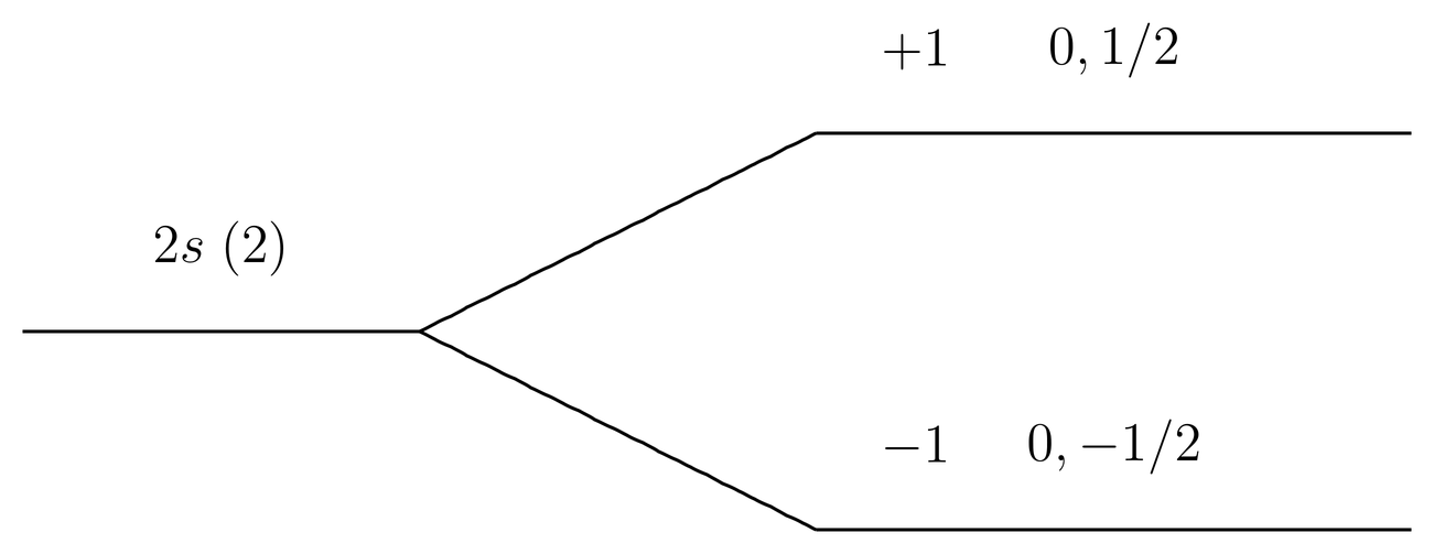
Figure 1:a. Strong field Zeeman splitting in level of hydrogen. The number in parentheses is the degeneracy of the unperturbed state. The energy shifts are measured in units of . The quantum numbers in the kets are , the other quantum numbers and being understood.
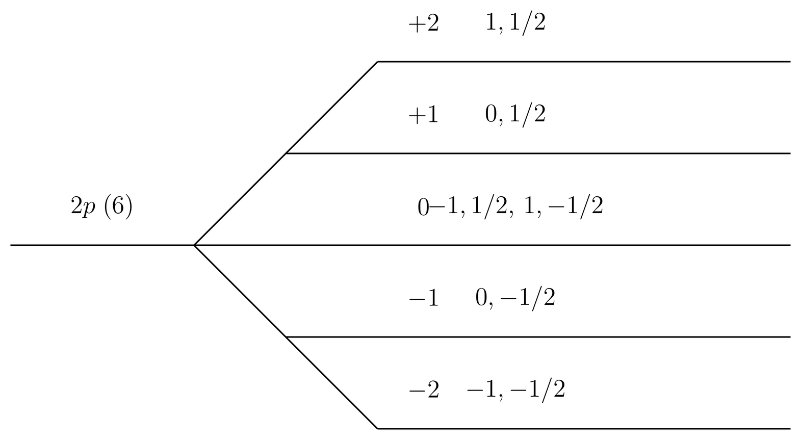
Figure 2:b. Same as Figure 1a, except for the level of hydrogen, which is 6-fold degenerate. The perturbed level is 2-fold degenerate. Quantum numbers and are understood.
Therefore the energy shifts are given by
In the final expression we have used (1), which makes the answer valid in both atomic and ordinary units, since has dimensions of energy. The results are displayed in Figure 1a for the set of states and in Figure 1b for the set of states of hydrogen. We see that the 2-fold degeneracy of the states is completely lifted by the perturbation, while the 6-fold degeneracy of the set of states is only partially lifted, with five equally spaced energy levels in the presence of the magnetic field, one of which is 2-fold degenerate.
Actually, Figs.~Figure 1 are valid for any or set of states, either in hydrogen or in an alkali. In hydrogen, however, notice that there is a further degeneracy, because the states in the set of states are degenerate with the states of the set. Altogether, of the 8 degenerate states of the the level of hydrogen in the unperturbed system, there are two nondegenerate levels () after the perturbation is turned on, and three 2-fold degenerate levels ().
Case II. , not Negligible
Now we consider the case that is much larger than the fine structure terms , as in Case I. Dominant, Negligible, but not so large that those corrections can be neglected. Thus we will take the new unperturbed Hamiltonian to be
with as a perturbation. Notice that this is the entire Hamiltonian of Case I. Dominant, Negligible.
More precisely, we will take to be the spin-orbit term only, and ignore the relativistic kinetic energy and Darwin corrections. This is not realistic, because all three fine structure terms are of the same order of magnitude, but we do it for simplicity. As for the spin-orbit term, we write
so that
In the following we concentrate mainly on hydrogen, with a few comments about the alkalis. Some of the eigenstates of are degenerate, as we have seen in Case I. Dominant, Negligible, so we must think about degenerate perturbation theory. We can only use the uncoupled basis, since the coupled basis is not an eigenbasis of . Thus we must look at the matrix elements
where we put primes to cover the degenerate eigenspaces of . For example, in the levels of hydrogen, we found in Case I. Dominant, Negligible that there were three 2-fold degenerate levels of (see Figs.~Figure 1a and Figure 1b). However, we see right away that , so the prime on is not necessary, and in fact we can carry out the perturbation analysis in subspaces of given separately. This is what we must do anyway in the case of the alkalis, where there is no degeneracy in in the unperturbed system. In the case of the levels of hydrogen, we see that we have only one 2-fold degeneracy, that between the and states. This makes one matrix. Let us look at the off-diagonal element,
in which we use the identity,
To be nonvanishing, the operator in the middle of the matrix element (22) must connect states with , but in fact that operator permits only or . Therefore the off-diagonal matrix element (22) vanishes, and, for the levels of hydrogen, we can use nondegenerate perturbation theory. Once again, there are no matrices to diagonalize.
Therefore to get the energy shifts we need only look at the diagonal matrix elements,
where we have used (23). The spin kets cancel each other in the final matrix element, which turns into a purely orbital matrix element of the type we saw previously in the treatment of the fine structure. See \finestruc.9. We have
where in the last step we have specialized to hydrogen. We use the expectation value (53), which is only valid for , to find
in the levels of hydrogen. As for the levels, for them (that is, the operator vanishes on the -subspace), so .
Case III: 
The final case we shall examine is the weak field limit, in which . Thus we take the unperturbed Hamiltonian and perturbation to be
In the case of hydrogen, one should also consider the Lamb shift for a realistic treatment. For example, in the levels of hydrogen, the Lamb shift is about 10 times smaller than the fine structure energy shifts, indicating that we really should question how the Lamb shift compares to the Zeeman term which is also (by our assumptions) much smaller than the fine structure term. For simplicity, however, we will ignore the Lamb shift in the following and work with (27) and (28).
The unperturbed energies are for hydrogen or for the alkalis, and the unperturbed eigenstates are members of the coupled basis . There is no option of using the uncoupled basis, which is not an eigenbasis of . The degeneracies are in the case of the alkalis, and more than this in hydrogen because of the degeneracy between different values. For example, the eight states of hydrogen consist of two levels, each 4-fold degenerate (see Fig.~\figr\finestruc.2). Thus we must think about degenerate perturbation theory.
In hydrogen the matrix elements we need have the form
where on the left we omit the primes on and since they define the unperturbed energy level , but put primes on the other two indices. In the case of the alkalis we do not need the prime on , since the unperturbed energies are . Actually, we do not need the prime on in the case of hydrogen, either, since . Nor for that matter do we need the prime on , since , and once again we escape from having to diagonalize any matrices. The energy shifts are
We write , so that this becomes
The final matrix element of is not entirely trivial to evaluate in a reasonably elegant manner. A technique that has been found to do this involves some results in angular momentum theory. We now make a digression to discuss these results, before returning to apply them to the weak field Zeeman effect.
The Projection Theorem
In this we adopt the general notation for a standard angular momentum basis, , which was used in 13. Representations of the Angular Momentum Operators and Rotations. Compared to the notation used in Case III: , the correspondences are
We begin with an identity due to Dirac. We let be any vector operator. Then we have the identity,
This identity can be proved by working with the definition (21). The proof will be left as an exercise. See Prob.~\prbrzeeman-1.
We sandwich both sides of Dirac’s identity (33) between the states and , in which the values are the same on both sides but the other indices are allowed to be different. We let , so that the left hand side of (33) is and its matrix element is
Therefore the matrix element of the right hand side of (33) between the same states vanishes, or,
Rearranging, we have
which is the projection theorem. It is useful in several applications in atomic physics. It has generalizations in which the values on the two sides of the matrix element are allowed to be distinct, but this simpler version is all we shall need for the application we shall consider.
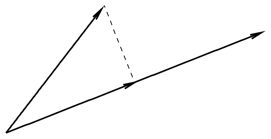
Figure 3:Geometrical meaning of the projection theorem.
The geometrical meaning of the projection theorem can be seen in Figure 2. If we think of and as classical vectors, then the projection of onto the direction is given by
On the other hand, the quantum projection theorem (36) states that the matrix elements of a vector operator on a subspace of a given are the same as the matrix elements of the projection (37), with the denominator reinterpreted as . The projection theorem can also be seen as an example of the Wigner-Eckart theorem, in which the reduced matrix element is explicitly evaluated.
The Weak Field Zeeman Effect
We now return to the matrix element of in (31), which we need for the energy shifts in the weak field Zeeman effect. We use the projection theorem with the identifications (32), and we also identify with . In this application of the projection theorem the states are the same on both sides of the matrix element, so we do not need the primes seen in (36). Thus we have
where we have taken the -component and reverted to atomic units. The operator brings out the quantum number when acting on the ket, while the operator can be put into a more useful form by expanding . This gives
Altogether, the matrix element becomes
and the energy shift (31) becomes
where
The dimensionless number is called the Land'e -factor.
It might seem surprising that the energy shifts should be proportional to , for while it is true that , the orbital and spin angular momentum do not contribute equally to the magnetic moment, due to the different -factors ( for orbital angular momentum, for electron spin, hence the expression in the Zeeman Hamiltonian). That is, the angular momentum operator is , while the magnetic moment operator is proportional to . Thus, is not proportional to . In 14. Spins in Magnetic Fields\ it was pointed out that in classical electrodynamics, the angular momentum and magnetic moment of a system are in general not proportional, and the question was left open why they should be so for a particle such as the nucleus of an atom. We see here that in atomic systems, too, the magnetic moment and angular momentum are not proportional. But the energy shifts (41) are the same as if the magnetic moment of the atom (orbital plus spin) were given by
a generalization of Eq. (12) (with ).
The reason for this is that all vector operators are proportional to any given vector operator on a single irreducible subspace under rotations. See Prob. Paragraph(a). The angular momentum is a convenient reference vector operator, so all vector operators, including , are proportional to on a single irreducible subspace. In the limit of weak magnetic field, the Zeeman Hamiltonian does not mix irreducible subspaces, that is, it only involves a single set of states with the same , and but with different , so the energy shifts are proportional to . For stronger fields, for example, one strong enough to overwhelm the fine structure splitting as in Case II. , not Negligible, the dependence of the energy levels on the magnetic quantum numbers is more complicated. The same would happen in a nucleus if the magnetic field were strong enough to mix more than one eigenspace of the nuclear Hamiltonian, although that would require extraordinarily large magnetic fields by ordinary standards.
Problems
Problem 1.
The projection theorem is useful in evaluating matrix elements for the Zeeman effect and for the hyperfine structure of hydrogen.
Show that if is a vector operator, then
Then use this to show that
where the notation of 13. Representations of the Angular Momentum Operators and Rotations\ is used.
Problem 2.
In this problem we aim to do a realistic calculation of the effect of magnetic fields on the states of hydrogen. (For simplicity we will set throughout.) We will allow the magnetic field to take on any value, so that we will not assume that the Zeeman term is necessarily small or large in comparison to the fine structure terms. (We will, however, ignore the Lamb shift.)
In these notes we have studied various limiting cases. In The Weak Field Zeeman Effect we studied the case that is so weak that the spin-orbit term dominates the Zeeman term. There we found (see (41) that the energy shifts were
where is the Land'e -factor,
Next, when is so strong that the spin-orbit term can be neglected (Case I. Dominant, Negligible), we found (17) for the energy shifts. Some books (e.g., Sakurai) do similar calculations, but they ignore the Darwin and relativistic kinetic energy corrections, which is not realistic because they are of the same order of magnitude as the spin-orbit term.
Consider therefore the Hamiltonian,
where
See (25), (28) and (13) for the definitions of these various terms. Take the magnetic field to point along the -axis, . The term is proportional to the applied field , which is a parameter of the perturbing Hamiltonian. You are to evaluate the corrections to the energy levels due to this perturbation, as a function of , using first-order perturbation theory. To simplify the notation, I suggest that you use atomic units throughout. Also, I recommend that you introduce the dimensionless variable to represent the strength of the magnetic field,
where
where is defined by (4). This definition is useful for the present problem, because it makes approximately the value for which the Zeeman term is comparable to the fine structure term.
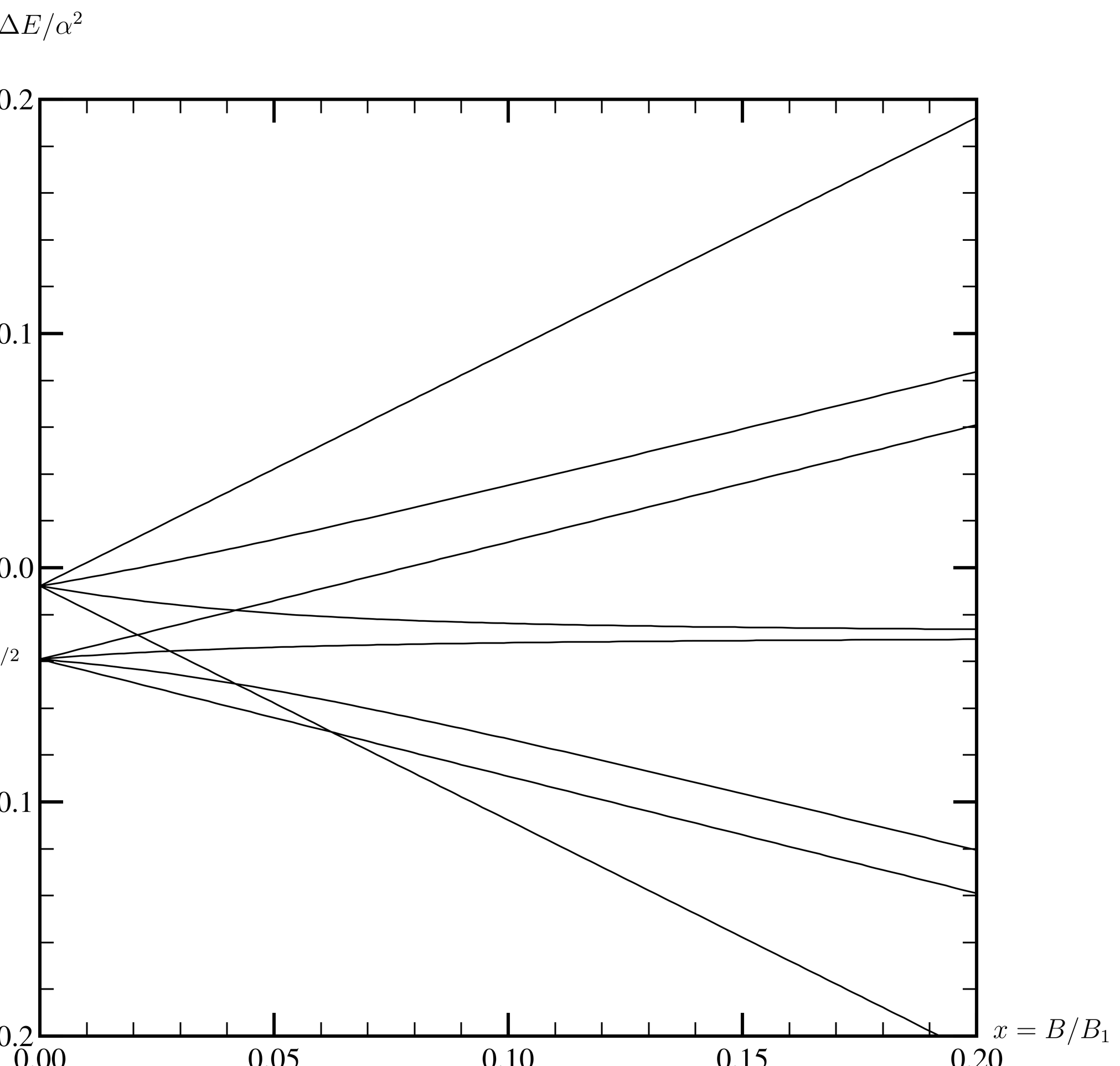
Figure 4:Graph of solutions to Prob. \prbrzeeman-2. The Zeeman energy shift is measured relative to the level of hydrogen in the electrostatic model, which is in atomic units. The fine structure energy shifts at zero field strength are for the and levels, where is the fine structure constant, and for the levels. The model ignores the Lamb shift, which is why the and levels are degenerate in the figure at zero field strength. Including the Lamb shift would modify the picture slightly.
(a) Out of the list of operators, , , , , , , , , , , , , , indicate which commute with and which commute with the entire Hamiltonian . Use this information to choose a convenient basis in the 8-dimensional subspace of the degenerate energy levels of , for which the perturbing Hamiltonian will be as diagonal as possible.
(b) Let be the difference between the true energy levels of (including the perturbation) and the 8-fold degenerate level of . Find all eight levels as a function of in atomic units.
(c) Expand these results out for small , and show that they agree with (46). Also expand the results for large , and show that the results agree with (17).
See Figure 3, a plot of the answers. The figure reveals a typical behavior of energy levels in various versions of the Zeeman effect. Notice that energy levels cross as the parameter (in this case, the magnetic field strength) is varied. Notice also that the fine structure splitting is overwhelmed by the Zeeman energy shifts at relatively small values of the parameter . We might have expected this to occur around , based on the scalings we have introduced, but the quantum numbers introduce additional dimensionless factors that reduce the value to something closer to , which corresponds to a magnetic field of about .
Problem 3.
This is another approach to the proof of the projection theorem, one which uses the Wigner-Eckart theorem. In the following we let and be vector operators, which for simplicity we assume to be Hermitian. This means that , , for all three Cartesian components of and .
(a) Since is a vector operator, the Wigner-Eckart theorem says
where . See The Spherical Basis for the spherical basis . Now let be a scalar operator. Then since is another vector operator, we must have
where just means the reduced matrix element for the vector operator . Also, since is a scalar, we have
where the Clebsch-Gordan coefficient is trivial since .
Show that
(b) For the special case , work out an explicit formula for the reduced matrix element, . Hint: Take the component, , and use (88) to evaluate the Clebsch-Gordan coefficient explicitly. Then solve for the reduced matrix element.
(c) Since and are vector operators, is a scalar operator. Express the reduced matrix element of the scalar in terms of the reduced matrix elements of and . Hint: Note that
where we use (11).
(d) Now show that
vanishes unless . In the case , work out the reduced matrix element in terms of the reduced matrix element of . Use this to show that
which is the projection theorem.
Problem 4.
The wave function of spin- particle can be considered to be a 2-component column spinor,
as in (16). Then the Hermitian conjugate wave function can be seen as a 2-component row spinor,
In this notation, the normalization integral can be written
(a) The magnetic moment operator of an electron is given by (16), and that of a neutron by (24). Find the expectation value of the magnetic moment operator for an electron and for a neutron, when the wave function satisfies , that is, the particle is polarized as “spin up.” Express your answer in terms of -factors and other physical constants.
In this case the expectation value of the magnetic moment vector has only a -component. We consider this -component to be “the magnetic moment” (that is, a scalar value) of the electron or neutron.
(b) Iron has a density of 7.87 , and an atomic weight of 55.8. Assuming each iron atom has an average of one electron aligned in the -direction, find the magnetization . (The magnetization is defined as the dipole moment per unit volume in both SI and Gaussian units. See Appendix~\emunits. The Gaussian unit of magnetization is , and the SI unit is , which is also an . One is the same magnetization as as .)
A uniformly magnetized sphere has a magnetic field given by
in Gaussian units. Compute the magnetic field strength inside a uniformly magnetized sphere of iron, under the assumptions of the previous paragraph.
Iron actually has four electrons whose spins can be aligned. If you multiply your answer by 4, you will get a value close to but somewhat larger than the practical saturation field strength in an iron core magnet. This number is important to experimentalists, for example, particle physicists who must bend particle beams with magnetic fields. To achieve much higher field strengths requires superconductors, which produce them by means of massive currents, without the aid of any substance of high permeability as a core.
(c) A neutron star has a density of . Find the magnetic field inside a uniformly magnetized sphere of such material, assuming each neutron is aligned with the magnetic field.
Problem 5.
The Land'e -factor gives the proportionality between and on a single irreducible subspace of the atomic Hilbert space with quantum numbers and . Given that the magnetic moment operator is proportional to , it would be logical that if then the Land'e -factor should become equal to the electron -factor, whereas if , then it should become equal to the -factor for orbital motion, which is 1. Show that this is true.
Problem 6.
The deuteron is a bound state of a proton and a neutron. It is the simplest compound nucleus. Here are the experimental facts.
The deuteron has only one bound state, the ground state, with energy . It has spin~1 and -factor,
The deuteron has an observed electric quadrupole moment.
We will model deuterium as a 2-body system consisting of a proton and a neutron. We make the approximation that the masses of the proton and neutron are equal. The proton and neutron both have spin and their -factors are
What we call the “spin” of the deuteron is really the total angular momentum of this 2-body system,
where is the orbital angular momentum of the relative motion of the 2-body system, and and are the spins of the proton and neutron. The ground state is an eigenstate of with quantum number , and is 3-fold degenerate with .
As explained in 14. Spins in Magnetic Fields, when a proton or neutron is placed in a magnetic field, there is an interaction energy given by or , respectively, where
The nuclear magneton is a convenient reference for measuring nuclear magnetic moments; it is defined by
which by convention uses the proton mass, even for the neutron and other particles. When the deuteron is placed in a weak magnetic field, its energy shift is proportional to ,
which serves to define , the deuteron -factor. It is like the Land'e -factor, which applies to atoms, but one difference is that even very powerful magnetic fields are “weak” by nuclear standards. Our problem will be to explain the observed value of in terms of a 2-body model of the deuteron.
(a) It is shown in Prob. Paragraph that the ground state of a central force problem is always an -wave (with ). If deuterium is a central force problem, then its one and only ground state must have . Then we can ignore in (65) and just concentrate on the spin degrees of freedom. (Take the Hilbert space to be just the product of the two spin Hilbert spaces, with .) The perturbing (Zeeman) Hamiltonian is just the interaction of the two spins with the magnetic field,
The spins must be in the triplet state, since we know that .
Use the projection theorem to find an expression for the -factor of the deuteron in this model. Evaluate the expression numerically.
(b) You should get an answer that is pretty good but not perfect. Call this answer , the first stab at a theoretical prediction of the -factor of the deuteron.
We conclude that the deuteron is not exactly a central force problem. But the calculation of part (a) shows that the ground state wave function of the deuteron is probably mostly an -wave (because the agreement is pretty good), but that there must be contributions from orbital angular momentum values . Mixing of different values in an energy eigenstate means that is not a good quantum number; if the system is not central force, then this is no surprise.
Hydrogen is not a central force problem, either, if we include the fine structure. We know that fine structure corrections are essentially relativistic, and are of order compared to nonrelativistic energies. Take the observed binding energy of the deuteron and assume it gives an estimate of the kinetic energy of the proton or neutron as they orbit one another. Use this to obtain an estimate of , and compare it to the of the electron in the ground state of hydrogen. Use this to estimate the momentum of the proton or neutron in its orbit around the other particle, and then use the uncertainty princple to estimate the radius of the orbit. You should find a value somewhat larger than the radius of the proton, which is about . This is because the deuteron is only weakly bound, and the wave function tunnels significantly into the classically forbidden region.
(c) Henceforth we must include the spatial degrees of freedom in our model, and we cannot ignore in (65). The orbital motion of the proton, a charged particle, must contribute to the magnetic moment of the deuteron.
Let be the normalized ground state of deuterium. This is an eigenstate of and with quantum numbers and , respectively. Project this onto the eigenspaces of , and call the projected vectors , where is normalized. That is, write
where
Use the experimental facts and the rules of angular momentum to determine which values may occur in this sum.
We have decided that . Given this and the fact that the strong interactions conserve parity, revise your list of allowed values. See Parity and Energy Eigenstates in Isolated Systems.
Show that the ground state is an eigenstate of , where
is the total spin of the proton-neutron system. Note that .
(d) In atoms, the Zeeman Hamiltonian is given by
a version of (13), which shows the -factors ( for orbital and for spin) of an electron.
In deuterium, we must take
that is, with an orbital factor of . This is because the orbital operator in deuterium includes the angular momentum of both the proton and the neutron about their common center of mass, while only the proton contributes to the orbital magnetic moment (because the neutron is neutral). This is where we use the approximation that the proton and neutron masses are equal; it hardly makes a difference for this problem.
Compute the energy shift in terms of the unknown coefficients . Assume , and notice that the term vanishes on an -wave. Explain why the cross terms vanish. For the other terms use the projection theorem, and choose your angular momentum carefully. Find an expression for in terms of the coefficients .
(e) Plug in the experimental value of and find the probability that the deuteron is not in an -wave. By the way, the nonvanishing electric quadrupole moment also shows that the deuteron is not purely an -wave.