34. Time-Dependent Perturbation Theory
Introduction
Time-dependent perturbation theory applies to Hamiltonians of the form
where is solvable and is treated as a perturbation. In bound state perturbation theory (see 23. Bound-State Perturbation Theory) we were interested in the the shifts in the energy levels and eigenfunctions of the unperturbed system induced by the perturbation , which was assumed to be time-independent. In time-dependent perturbation theory, on the other hand, we are usually interested in time-dependent transitions between eigenstates of the unperturbed system induced by the perturbation . In time-dependent perturbation theory the perturbation is allowed to depend on time, as indicated by (1), but it does not have to be time-dependent, and in fact in practice often it is not. Time-dependent perturbation theory is especially useful in scattering theory, problems involving the emission and absorption of radiation, and in field theoretic problems of various kinds. Such problems will occupy us for the rest of the course.
Time-dependent transitions are usually described by the transition amplitude, defined as the quantity
where is the exact time evolution operator for the Hamiltonian (1), and where and are two eigenstates of the unperturbed Hamiltonian (the “initial” and “final” states). The transition amplitude can be regarded as simply a matrix element of the exact time evolution operator in the eigenbasis of the unperturbed Hamiltonian, but it is also the amplitude to find the system in state when it was known to be in the state at . Thus, the absolute square of the transition amplitude is the transition probability, the probability to make the transition in time . Often we are interested in transitions to some collection of final states, in which case we must sum the transition probabilities over all these states.
In these notes we shall develop the basic formalism of time-dependent perturbation theory and study some simple examples. For the most part we shall simply follow the formulas to see where they lead, without examining the conditions of validity or the limitations of the results. We will address those questions in the context of some examples, both in these and in successive notes.
Time-Evolution Operators
Let us denote the unperturbed time-evolution operator by and the exact one by . Since the full Hamiltonian may depend on time, the exact time-evolution operator actually depends on two times, and , but we shall set and just write . See The Time-Evolution Operator. These operators satisfy the evolution equations,
which are versions of (13). Since is independent of time, (3) can be solved,
but if depends on time then there is no similarly simple expression for .
The Interaction Picture
The interaction picture is a picture that is particularly convenient for developing time-dependent perturbation theory. It is intermediate between the Schr"odinger and Heisenberg pictures that were discussed in The Heisenberg Picture. Recall that in the Schr"odinger picture, the kets evolve in time but the operators do not (at least if they have no explicit time dependence), while in the Heisenberg picture the kets do not evolve but the operators do. In the interaction picture, the time evolution of the kets in the Schr"odinger picture that is due to the unperturbed system is stripped off, leaving only the evolution due to the perturbation . This is presumably slower than the evolution due to the whole Hamiltonian , since is assumed small compared to . We will not attempt to state precisely what “small” means in this context, rather we will develop the perturbation expansion as a power series in and then examine its limitations in various examples.
In the following we shall use an subscript on kets and operators in the Schr"odinger picture, and an on those in the interaction picture. We will not use the Heisenberg picture in these notes. If the subscript is omitted, the Schr"odinger picture will be assumed. The the relation between the kets in the Schr"odinger and interaction pictures is
Compare this to (17), which shows the relation between kets in the Schr"odinger and Heisenberg pictures. The difference is that in (6) we are only stripping off the evolution due to , not the whole time evolution. Notice that at the Schr"odinger and interaction picture kets agree,
As for operators in the interaction picture, they are defined by
In practice is often time-independent, but is always time-dependent. Compare this to (19), which shows the relation between operators in the Schr"odinger and Heisenberg pictures.
Evolution in the Interaction Picture
Let us define as the operator that evolves kets in the interaction picture forward from time 0 to final time :
The operator is a time-evolution operator, but we use the symbol to avoid confusion with the two other time-evolution operators introduced so far, and .
It is easy to find a relation among these three operators. Substituting (6) and (7) into (9), we have
or, since is arbitrary,
The operator is equivalent to first evolving forward for time under the exact Hamiltonian, then evolving backwards for the same time under the unperturbed Hamiltonian.
The -Matrix
For an application in which the interaction picture leads to a interesting perspective, consider a scattering experiment in which a wave packet is directed against a target, described by a potential . We assume that the potential dies off rapidly with distance, and that at the initial time the wave packet is far enough away from the scatterer that it is essentially free. For simplicity we assume that the potential (or other perturbing Hamiltonian) is time-independent.
Initially the wave packet evolves according to the free particle Hamiltonian, since it does not overlap with the potential. That is, the wave packet moves with an average velocity and simultaneously spreads, as studied in Prob. Paragraph. After some time, however, the wave packet begins to interact with the potential, producing a scattered wave that radiates outward from the potential in various directions. Depending on the size of the wave packet and that of the scatterer, some of the wave packet may effectively miss the scatterer and proceed in the forward direction, largely unaffected by the scattering process. In any case, after some time the scattered wave and the remaining part of the incident wave packet move away from the scatterer, and once again evolve according to the free particle Hamiltonian. Thus, the exact time evolution is that of a free particle both at large negative times and large positive times.
Let us now view the evolution of the quantum state in the interaction picture. Initially and for large negative times the wave function in the Schr"odinger picture evolves according the free particle Hamiltonian, so in the interaction picture the wave function does not evolve at all. The wave function in the interaction picture does not begin to change until the wave packet in the Schr"odinger picture starts to interact with the potential. Then the wave packet in the interaction picture does evolve, and continues to do so as long as the Schr"odinger wave function has any overlap with the scatterer. As the Schr"odinger wave function leaves the region of the scatterer, however, the wave function in the interaction picture ceases to evolve, and at large positive times it approaches another, constant wave function.
Thus, the interaction picture kets and approach constant kets as . The scattering process associates a given initial state with a definite final state . This association is linear, and defines the -matrix. It is usually called a “matrix” but really it is an operator, whose matrix elements in some basis form a matrix. The usual basis is that of free particle states, that is, plane waves. In this form, the -matrix bears a close relationship to the cross .
We can easily express the -matrix (or operator) in terms of time-evolution operators. Since
we have
But
where we have used and . But by the definition of the operator, this implies
The -matrix is a central object in advanced treatments of scattering theory, but its mathematics involves noncommuting limits and is tricky. In these notes we take a simpler approach to scattering theory, one that involves a straightforward perturbation expansion of the operator in powers of the perturbing Hamiltonian .
The Dyson Series
We obtain a differential equation for by differentiating (11) and using (3),
where we have used in the third equality, whereupon the terms in cancel. The result can be written,
an equation of the same form as (3), but one in which only the perturbing Hamiltonian appears, and that in the interaction picture. By applying both sides of (18) to the initial state , we obtain a version of the Schr"odinger equation in the interaction picture,
It is now easy to obtain a solution for as a power series in the perturbing Hamiltonian . First we integrate (18) between time 0 and time , obtaining
where we have used . This is an exact result, but it is not a solution for , since appears on the right-hand side. But by substituting the left-hand side of (20) into the right-hand side, that is, iterating the equation, we obtain
another exact equation in which the term containing on the right hand side has been pushed to second order. Substituting (20) into the right-hand side of (21) pushes the term in to third order, etc. Continuing in this way, we obtain a formal power series for ,
This series is called the Dyson series. It is obviously a kind of a series expansion of in powers of .
The Usual Problem
Let us assume for simplicity that has a discrete spectrum, and let us write
where is a discrete index. The usual problem in time-dependent perturbation theory is to assume that the system is initially in an eigenstate of the unperturbed system, what we will call the “initial” state with energy ,
This is just a special case of (23) (with ). That is, we assume the initial conditions are
We will be interested in finding the state of the system at a later time,
By applying the Dyson series (22) to this equation, we obtain a perturbation expansion for ,
Transition Amplitudes
Let us expand the exact solution of the Schr"odinger equation in the interaction picture in the unperturbed eigenstates,
with coefficients that are functions of time. We can solve for these coefficients by multiplying (28) on the left by the bra , which gives
showing that is a transition amplitude in the interaction picture, that is, a matrix element of the time-evolution operator in the interaction picture with respect to the unperturbed eigenbasis. These are not the same as the transition amplitudes (2), which are the matrix elements of (the time-evolution operator for kets in the Schr"odinger picture) with respect to the unperturbed eigenbasis. There is, however, a simple relation between the two. That is, substituting (11) into (29), we have
where we have allowed to act to the left on bra . We see that the transition amplitudes in the interaction picture and those in the Schr"odinger picture are related by a simple phase factor. The phase factor removes the rapid time evolution of the transition amplitudes in the Schr"odinger picture due to the unperturbed system, leaving behind the slower evolution due to . The transition probabilities are the squares of the amplitudes and are the same in either case,
The perturbation expansion of the transition amplitude is easily obtained by multiplying (27) by the bra . We write the result in the form,
where the parenthesized numbers indicate the order of perturbation theory, and where
etc.
We now switch back to the Schr"odinger picture in the expressions for the . The interaction picture is useful for deriving the perturbation expansion, but the Schr"odinger picture is more convenient for subsequent calculations. For , we have
where we have allowed and to act to the left and right, respectively, on bra and ket , bringing out the phase factor where is the Einstein frequency connecting unperturbed states and ,
As for , it is convenient to introduce a resolution of the identity between the two factors of in (34) before switching to the Schr"odinger picture. This gives
From this the pattern at any order of perturbation theory should be clear. In (38), the states are known as intermediate states, the idea being that there is a time sequence as we move from the right to the left in the product of matrix elements, starting with the initial state , moving through the intermediate state and ending with the final state . Notice that the variables of integration satisfy .
The Case that is Time-independent
This is about as far as we can go without making further assumptions about , so that we can do the time integrals. Let us now assume that is time-independent, an important case in practice. Then the matrix elements are independent of time and can be taken out of the integrals, and the integrals that remain are elementary. For example, in (36) we have the integral
so that
The case of is similar but more complicated. We will return to it in 43. Scattering of Radiation by Matter{} when we apply second order time-dependent perturbation theory to the problem of the scattering of photons.
The transition probability can also be expanded in the perturbation series,
Notice that on taking the square there are cross terms, that is, interference terms between the amplitudes at different orders.
For now we assume that the final state we are interested in is not the the initial state, that is, we take the case so the first term in (41) vanishes, and we work only to first order of perturbation theory. Then we have
The transition probability depends on time and on the final state . As for the time dependence, it is contained in the first factor in the parentheses, while both this factor and the matrix element depend on the final state . However, the factor in the parentheses depends on the state only through its energy , which is contained in the Einstein frequency , while the matrix element depends on all the properties of the state , for example, its momentum, spin, etc.
The case is interesting, too, as it gives the amplitude and probability for the system to remain in the initial state. This case will be analyzed in some detail in 44. Natural Line Width, Long-Time Behavior and the Lamb Shift.
The Case of Time-Periodic Perturbations
Another case that is important in practice is when has a periodic time dependence of the form
where is the frequency of the perturbation and is an operator (generally not Hermitian). We call the first and second terms in this expression the positive and negative frequency components of the perturbation, respectively. This case applies, for example, to the interaction of spins or atoms with a given, classical electromagnetic wave, a problem that is studied in 35. The Photoelectric Effect.
To find the transition amplitude in this case we substitute (43) into (36) and perform the integration, whereupon we obtain two terms,
For any given final state , both these terms are present and contribute to the transition amplitude, and when we square the amplitude to get the transition probability, there are cross terms (interference terms) between these two contributions to the amplitude.
Often, however, we are most interested in those final states to which most of the probability goes, which are the states for which one or the other of the two denominators in (45) is small. For these states we have , or
We see that the first (positive frequency) term is resonant when the system has absorbed a quantum of energy from the perturbation, whereas the second (negative frequency) term is resonant when the system has given up a quantum of energy to the perturbation. We call these two cases absorption and stimulated emission, respectively.
Taking the case of absorption, and looking only at final states that are near resonance (), we can write the transition probability to first order of perturbation theory as
Similarly, for nearly resonant final states in stimulated emission, we have
These formulas may be compared to (42). In all cases, has a dependence on time that is described by functions of a similar form.
How Depends on Time
Let us fix the final state and examine how the probability develops as a function of time in first order time-dependent perturbation theory. To be specific we will take the case of a time-independent perturbation and work with (42), but with replaced by and replaced by or , everything we say also applies to absorption or stimulated emission.
Obviously (because and all the probability lies in state at ). At later times we see that oscillates at frequency between 0 and a maximum proportional to . The frequency measures how far the final state is “off resonance,” that is, how much the final energy differs from the initial energy. In some applications this difference can be regarded as a failure to conserve energy, which is allowed over finite time intervals by the energy-time uncertainty relation . If is large, the probability oscillates rapidly between zero and a small maximum. But as we move the state closer to the initial state in energy, gets smaller, the period of oscillations becomes longer, and the amplitude grows.
If there is a final state degenerate in energy with the initial state (not the same state since we are assuming ), then and the time-dependent factor in (42) takes on its limiting value, which is . In this case, first order perturbation theory predicts that the probability grows without bound, obviously an absurdity after a while since we must have . This is an indication of the fact that at sufficiently long times first order perturbation theory breaks down and we must take into account higher order terms in the perturbation expansion. In fact, to get sensible results at such long times, it is necessary to take into account an infinite number of terms (that is, to do some kind of summation of the series). But at short times it is correct that for a state on resonance grows as .
These considerations are important when the system has a discrete spectrum, for example, when a spin is interacting with a time-periodic magnetic field or when we are looking at a few discrete states of an atom in the presence of laser light. These are important problems in practice. Recall that in 14. Spins in Magnetic Fields\ we solved the Schr"odinger equation exactly for a spin in a certain kind of time-periodic magnetic field, but in more general cases an exact solution is impossible and we may have to use time-dependent perturbation theory. It is interesting to compare the exact solution presented in 14. Spins in Magnetic Fields\ with the perturbative solutions presented here, to see the limitations of the perturbative solutions.
In such problems with a discrete spectrum, the resonance condition may not be satisfied exactly for any final state . In fact, in problems of emission and absorption, if the frequency of the perturbation is chosen randomly, then it is unlikely that the resonant energy will exactly coincide with any unperturbed energy eigenvalue. In that case, first-order theory predicts that the transition probability to all final states just oscillates in time.
On the other hand, if the final states are members of a continuum, then there are an infinite number of final states arbitrarily close to the initial state in energy. For those cases, we must examine how the transition probability depends on energy.
How Depends on Energy
Now let us fix the time and examine how the expression for in first order perturbation theory, (42), depends on the energy of the final state (working for simplicity with the case of a time-independent perturbation). We shall concentrate on the energy dependence of the time-dependent factor in the parentheses, remembering that the matrix element also depends on the energy (and other parameters) of the final state. To do this we plot the function as a function of , as shown in Figs.~Figure 1 and Figure 2 for two different times. In the plot, is to be identified with , so that specifies the energy of the final state and is the resonance (energy conserving) condition.
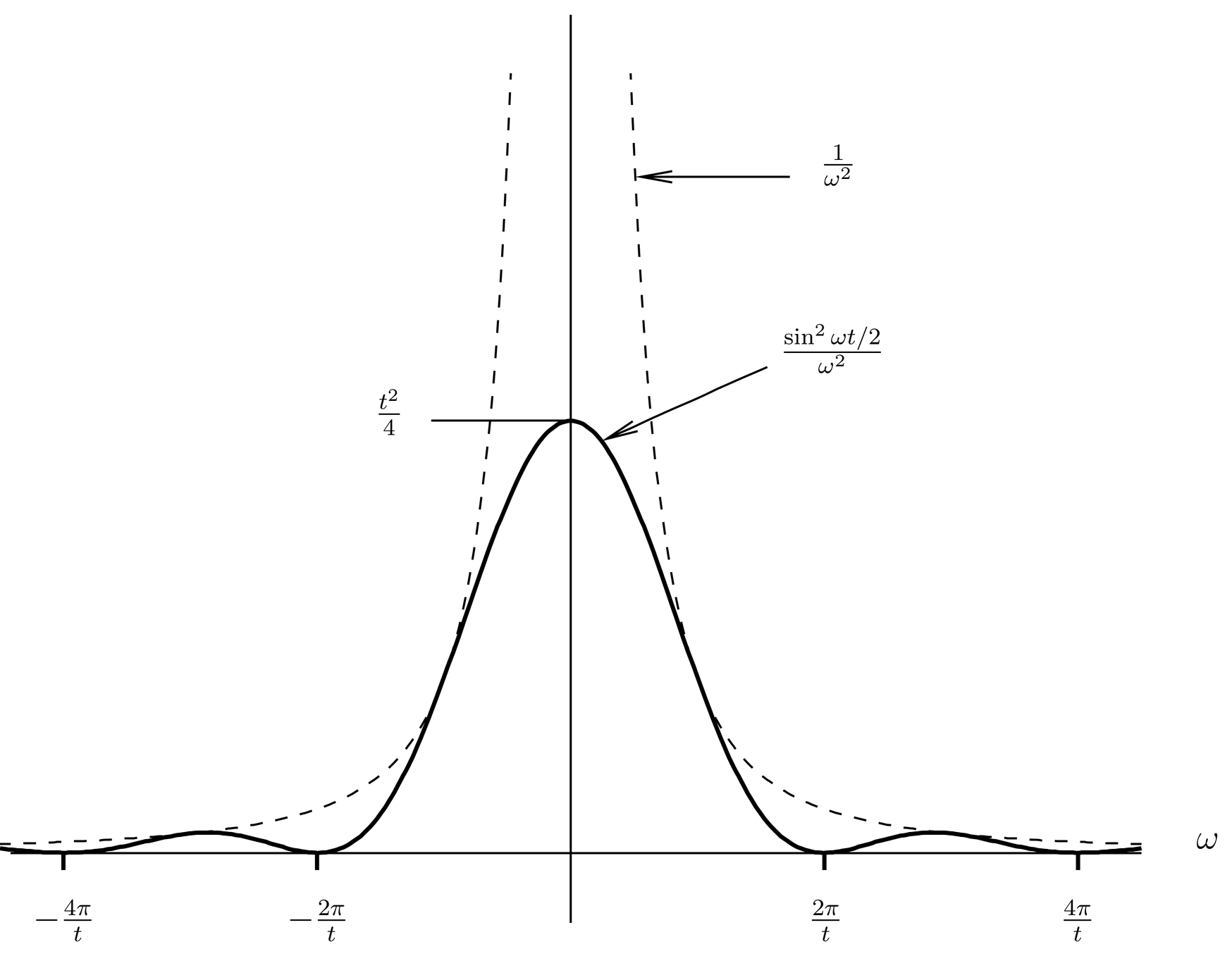
Figure 1:The function as a function of for fixed . The dotted curve is the envelope .
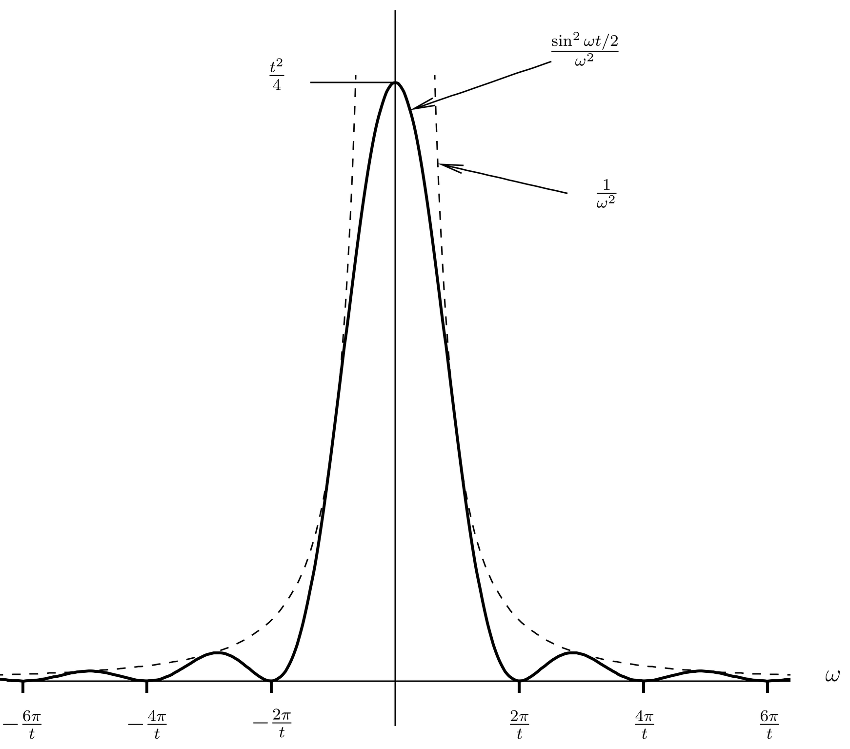
Figure 2:Same but for a larger value of . The area of the curve is dominated by the central lobe, and grows in proportion to .
The curve consists of oscillations under the envelope , with zeroes at . The central lobe has height and width that is proportional to , so the area of the central lobe is proportional to . As increases, the central lobe grows in height and gets narrower, a behavior that reminds us of functions that approach a -function, but in this case the limit is not a -function because the area is not constant. In fact, the total area is given exactly by an integral that can be evaluated by contour integration,
showing that the area is indeed proportional to . Thus if we divide by we do get a -function as ,
For fixed the function under the limit in this expression approaches 0 as , while exactly at it grows in proportion to , with a constant total area. This is exactly the behavior that produces a -function in the limit.
In physical applications we never really go to infinite time, rather we work with times long enough that there is negligible error in replacing the function on the left-hand side of (50) by its limit. To deal with the case of finite time, we introduce the notation,
which defines the function . Then the limit (50) can be written,
As we shall see when we take up some applications, the -function in (50) enforces energy conservation in the limit , that is, only transitions to final states of the same energy as the initial state are allowed in that limit. At finite times, transitions take place to states in a range of energies about the initial energy, given in frequency units by the width of the function . But as we have seen this width is of order , or, in energy units, . This is an example of the energy-time uncertainty relation, , indicating that a system that is isolated over a time interval has an energy that is uncertain by an amount .
Now we can write the transition probability (42) as
This applies in first order perturbation theory, in the case .
Cross and Differential Cross In preparation for applications to scattering, we make a digression to define and discuss cross s and differential cross s. These concepts are best understood in a classical context, but most of the ideas carry over without trouble into quantum mechanics.
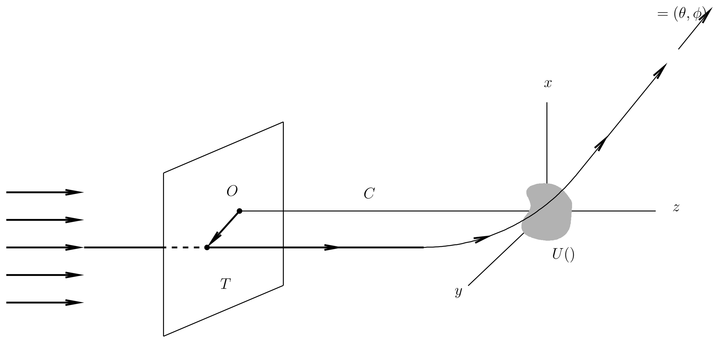
Figure 3:Classical scattering of particles. The outgoing asymptotic direction is a function of the impact parameter .
We first discuss classical scattering from a fixed target, which is illustrated in Figure 3. An incident beam of particles of momentum and uniform density is directed against a target, illustrated by the shaded region in the figure. The target is described by a potential . The origin of a coordinate system is located in or near the target, and in the figure the beam is directed in the -direction. A transverse plane is erected perpendicular to the beam at a large, negative value of , where the potential is negligible. The plane is parallel to the - plane, and when the particles cross it their momentum is purely in the -direction, since no interaction with the potential has occurred yet. The negative -axis is extended back to the plane along a center line , intersecting it at point , which serves as an origin in the plane.
The trajectory of one particle is illustrated in the figure. It crosses the plane at a position described by the impact parameter, a vector , which goes from the origin in the plane to the interpoint. The impact parameter only has - and -components. The particle continues forward and interacts with the potential, going out in some direction . This direction is defined asymptotically, that is, it is the direction of the particle’s momentum when it is once again at a large distance from the target. The outgoing direction is a function of the impact parameter,
which can be determined by integrating the equations of motion from given initial conditions on the plane .
(54) defines a mapping from the transverse plane to the unit sphere of outgoing directions, and the differential cross is closely related to the Jacobian of this map. That is, is the ratio of an infinitesimal area element in to a corresponding infinitesimal solid angle on the sphere.
To visualize this in more detail, we construct a small cone of solid angle , centered on the outgoing direction , as illustrated in Figure 4. The particles whose asymptotic, outgoing directions lie inside this cone cross the plane inside an area indicated by the shaded area in plane in the figure. This area represents the portion of the incident flux of particles that is directed into the small cone by the scattering process. It defines the *differential cross * by the formula,
The differential cross is a function of .
It is possible that more than one impact parameter will lead to the same final outgoing direction , for example, depending on a particle may orbit the target one or more times before emerging in a definite final direction. In that case the area in (55) should be replaced by a sum of areas, each corresponding to the same small solid angle in the outgoing direction.
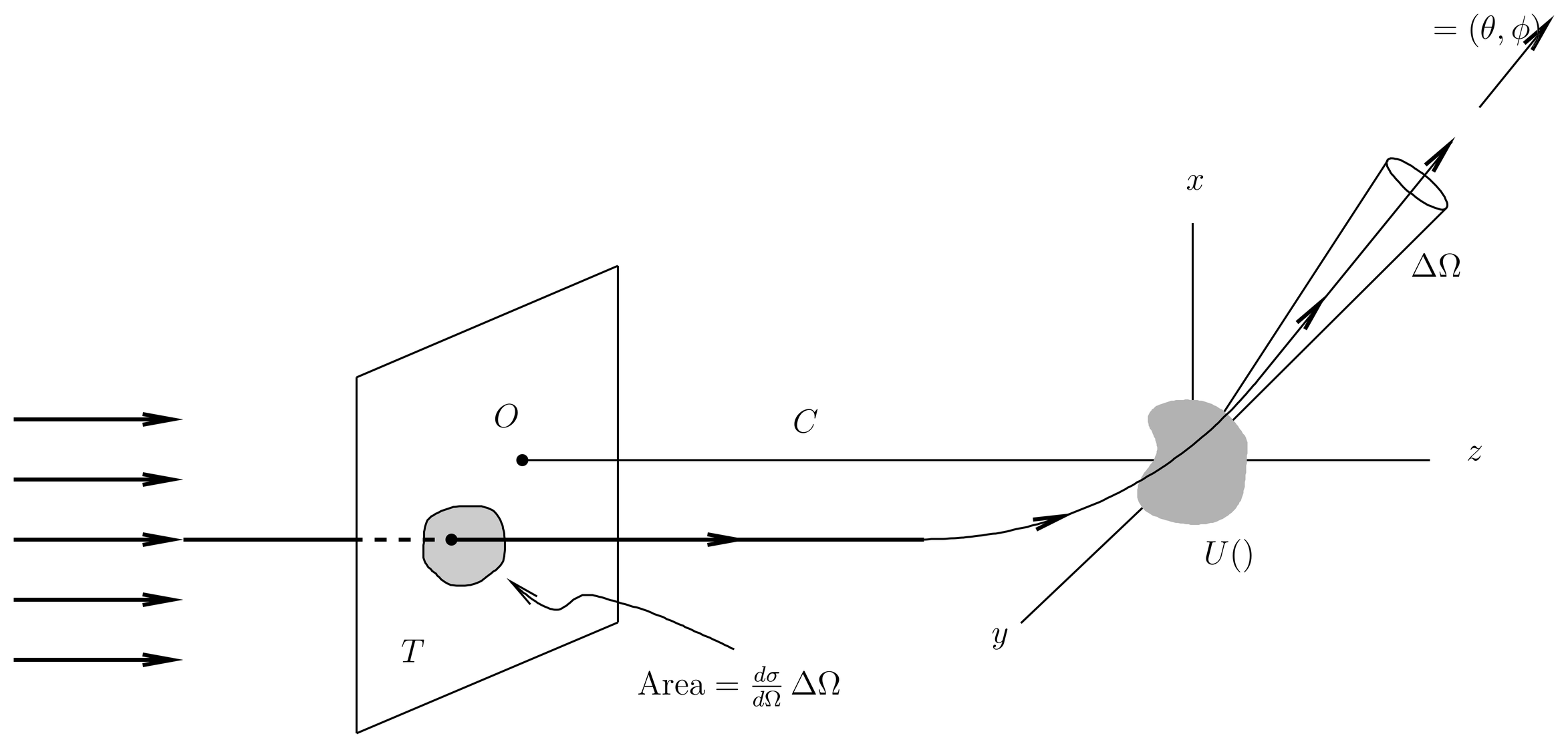
Figure 4:A subset of particles goes out into a small cone of solid angle centered on the direction . They cross the plane inside an area which is .
Another point of view deals with counting rates. We use the symbol to stand for a rate, with dimensions of , for example, number of particles per unit time or probability per unit time. A detector situated in Figure 4 so as to intercept all particles coming out in the cone will have a counting rate given by the rate at which particles cross the shaded area in plane . We denote this counting rate by . But this is just the flux of incident particles times the shaded area, that is,
As for the incident flux, it is given by
where is the number of particles per unit volume in the incident beam and is the incident velocity. The magnitude appears in (56), since the transverse plane is orthogonal to the velocity . It is obvious that the counting rate is proportional to the incident flux, so (56) gives another way of thinking about the differential cross : It is the counting rate, normalized by the incident flux.
The total scattering rate is the rate at which particles are scattered at any nonzero angle. It is the integral of the differential scattering rate,
It is related to the total cross by
where
In classical scattering, the total cross is often infinite, due to a large number of particles that are scattered by only a small angle.
The relation (56) applies in the case of a single scatterer located inside the incident beam. In many practical circumstances there are multiple, identical scatterers. An example is Rutherford’s scattering experiment, in which a beam of -particles is directed against a gold foil. The individual gold nuclei are the scatterers, of which there are a large number in the region of the foil crossed by the beam.
In this case we can speak of the scattering rate (differential or total) per unit volume of the scattering material, which is times the cross (differential or total), where and are the number of incident particles and scatterers per unit volume, respectively. Then integrating over the interaction region, we find that (56) is replaced by
where is again the velocity of the beam. In this formula, both and can be functions of position, as they often are in practice. We are assuming that is constant, so that it can be taken out of the integral (the beam consists of particles of a given momentum).
Another case that is common in practice is when there are two beams intersecting one another. In this case it is easiest to work in the center-of-mass frame, in which the momenta of the particles in the two beams are equal and opposite. As we have seen in 16. Central Force Motion, when two particles interact by means of a central force potential, their relative motion is described by a pseudo-one-body problem. Thus, the results for scattering from a fixed target with central force potential can be transcribed into those for scattering of two particles in the center of mass frame, in which the position vector of the beam particle relative to the scatterer is replaced by , the relative position vector between two particles in the two beams, and where the mass of the beam particle is replaced by the reduced mass of the two particle system. Then the transition rate is given by a modified version of (61),
where and are the densities of the two beams, which may be functions of position, and where is now the relative velocity of the two beams. The integral is taken over the region where the two beams overlap.
The transformation between the lab positions and momenta of the two particles, and , and the center of mass position and momentum and the relative position and momentum , is given by Eqs.~((44){}--(45)) and ((50){}--(53)). The definitions of , the center of mass position, and , the total momentum of the two particle system as seen in the lab frame, are clear physically. So also is the definition of , the relative separation between the two particles. But the definition of , the momentum conjugate to ,
requires some comment. (This is essentially (53).
We offer two interpretations of this equation. First, we compute , where is the reduced mass, given by (58), or, equivalently,
Dividing this into (63) gives
or,
where
is the relative velocity. In other words, we have a version of the usual formula , where is the momentum conjugate to the relative position vector, is the relative velocity, and is replaced by the reduced mass.
Another interpretation is to imagine the two particle system as seen in the center-of-mass frame, in which . If we let , then , which when substituted into (63) gives . Thus, the momentum , defined as the conjugate to the relative position , or, equivalently, by (63), is in fact the momentum of one or the other of the particles (to within a sign) as seen in the center-of-mass frame.
Application: Potential Scattering
We return now to time-dependent perturbation theory, and examine an application, namely, potential scattering of a spinless particle from a fixed target, described by a potential . We let the unperturbed Hamiltonian be and we take the perturbation to be , where is some potential. We do not assume the potential is rotationally invariant, but it should approach zero sufficiently fast as . We will examine this condition more carefully in Asymptotic Form of the Radial Wave Functions.
The unperturbed eigenstates are free particle solutions, which we take to be plane waves. In order to deal with discrete final states, we place our system in a large box of side and volume , and we adopt periodic boundary conditions. This is equivalent to dividing the universe up into boxes and demanding that all the physics be periodic, that is, the same in all the boxes. We shall assume that the size of the box is much larger than the range of the potential . When we are done we take to get physical results. We denote the unperturbed eigenstates by , with wave functions
so that
Here we are normalizing the eigenfunctions to the volume of the box, and integrating over the volume of the box when forming scalar products as in (69). The quantized values of are given by
where is a vector of integers, each of which ranges from to . The unperturbed eigenstates can be represented as a lattice of points in -space, in which the lattice spacing is and the density is . We let be an incident plane wave (the initial state), and be some final state.
Notice that the initial state is somewhat unrealistic from a physical standpoint. The initial state is a plane wave that fills up all of space, including the region where is appreciably nonzero. Let us suppose it is a potential well. Thinking in classical terms, it is as if all of space is filled with particles with exactly the same momentum and energy, even the particles in the middle of the well. Of course a particle coming in from infinity and entering a potential well will gain kinetic energy, and the direction of its momentum will change (this is the scattering process in action). But the particles of our initial state in the middle of the potential have the same kinetic energy and momentum as the particles that are coming in from infinity. Obviously this initial condition would be difficult to establish in practice. Nevertheless, it turns out that these particles with the wrong energy and momentum in the initial state do not affect the transition probabilities after sufficiently long times, and so they do not affect the cross that we shall compute. All they do is give rise to short-time transients that can be regarded as nonphysical since they arise from the artificialities of the initial conditions. We shall say more about these transients below, but for now we shall just continue to follow the formulas of time-dependent perturbation theory.
In this application the perturbing Hamiltonian is time-independent, so the transition amplitude in first order perturbation theory is given by (40), with the change of notation , , etc. The transition amplitude is
where
and the transition probability is
where we sum over some set of final states for which . Note that (72) implies
where is the classical velocity of the beam particles. It is also the group velocity of free particle wave packets.
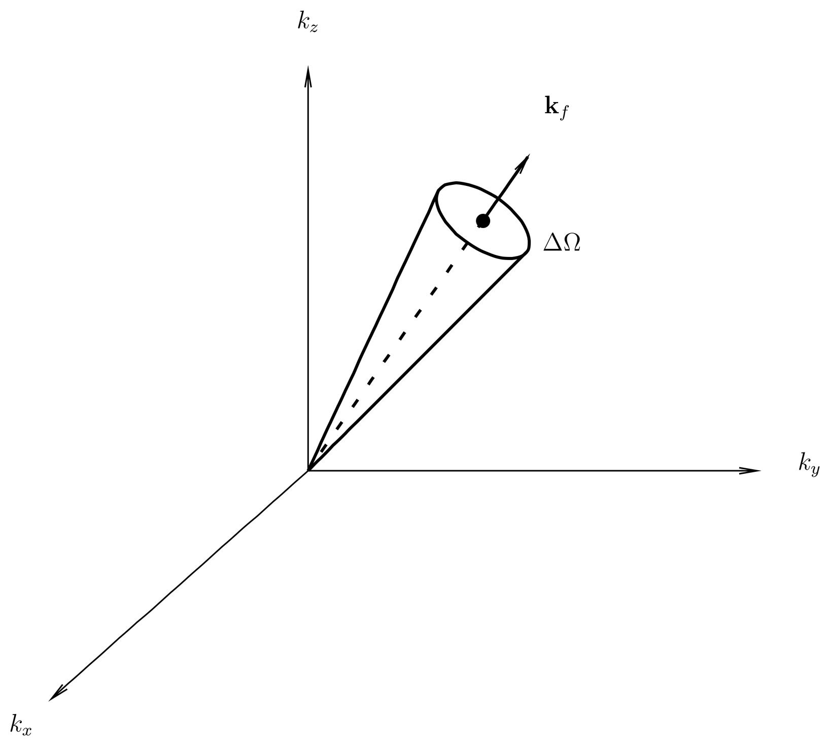
Figure 5:To compute the differential transition rate , we sum over all lattice points in -space lying in a small cone of solid angle centered on some final vector of interest. The direction of determines the dependence of the differential cross .
Which final states do we sum over? This depends on what question we wish to ask. If we are interested in the transition rate to any final state, then we sum over all of them (every lattice point in -space except ). Often, however, we are interested in more refined information. In the present case, let us sum over all final states (lattice points) that lie in a cone of small solid angle in -space, as illustrated in Figure 5. Let the cone be centered on a direction , a given unit vector pointing toward some counting device in a scattering experiment. Then we define a “final wave vector” by requiring that have the same direction as , and that it satisfy conservation of energy,
that is, . Then
This is only a definition, and although satisfies energy conservation, notice that the states in the cone that we sum over include states of all energies, from 0 to .
With this understanding of the states we sum over in the expression (73), we see that we are computing the probability as a function of time that the system will occupy a momentum state lying in the cone. Under some circumstances transition probabilities are proportional to time, and then we can refer to a transition rate as the probability per unit time for the process in question. We will generally use the symbol for transition rates. In the present case, we divide the probability (73) by and write
where is the transition rate per unit solid angle, a quantity that is generally a function of direction, in this case, the direction .
Notice that the factors of have canceled in (77), but the right-hand side still depends on through . If, however, is large enough that can be replaced by , then the right hand side does become independent of , and the transition rate is meaningful. We see that at short times we do not have a transition rate, but that at longer times we do.
For now let us assume that is large enough that can be replaced by , since this gives the simplest answer. This condition will be examined quantitatively in Short-Time Behavior. Then using (72), we can transform by the rules for -functions,
where we use (74).
We must also take the limit to obtain physical results. In this limit, the initial wave function loses meaning (it goes to zero everywhere, since it is normalized to unity over the volume of the box), as does the differential transition rate . However, the differential cross , which is the differential transition rate normalized by the incident flux, is well defined in the limit. The incident flux is
where is the number of particles per unit volume in the incident state, and is the incident velocity. Thus
Also, in the limit , the sum over lattice points in (77) can be replaced by an integral,
where is the density of states per unit volume in -space and where we have switched to spherical coordinates in -space and done the angular integral over the narrow cone.
Finally we evaluate the matrix element in (77). It is
where we use (68) and define the Fourier transform of the potential by
Putting all the pieces together, we have
where the factors of and have canceled, as they must. Notice that under the integral is a vector, but only its magnitude is a variable of integration. The direction of is that of the small cone, that is, . Now the -function makes the integral easy to do. In particular, becomes . Notice that if is large enough to make the replacement but not infinite, the function should be understood as a function of small but nonzero width. Thus after finite time the transitions are actually taking place to states that lie in a small energy range about the initial energy. This is an important point: in time-dependent perturbation theory, we do not attempt to enforce energy conservation artificially, rather our job is to solve the Schr"odinger equation, and when we do we find that energy conservation emerges in the limit .
The final answer is now easy. It is
Notice that the momentum transfer in the scattering process is
and the differential cross is a function of this momentum transfer. This result from first-order time-dependent perturbation theory is the same as that obtained in the first Born approximation, which we take up in 38. The Lippmann-Schwinger Equation and Formal Scattering Theory.
The result (86) is valid in the high-energy limit, in which the exact wave function in the midst of the potential does not differ much from the unperturbed wave function. This condition will be examined quantitatively in Conditions of Validity of the Born Approximation. This makes crude sense: since the Hamiltonian is , if the kinetic energy of the incident particles is large then in a sense we have , and an expansion of the transition amplitude in powers of should be valid. But high energy particles blast through the potential without being deflected very much. At low energies a naive power series expansion in powers of will not work, and other techniques are needed. Some of these are explored in 36. Introduction to Time-Independent Scattering Theory and Scattering from Central Force Potentials{} and \lippschw.
Short-Time Behavior
Let us now estimate the time after which the replacement becomes valid. Let us call this time , which we shall estimate as an order of magnitude.
The function has a width in given by , as an order of magnitude, or, in energy units, . We can convert this to wavenumber units by using
where we use (74). This is the width in the variable of the function we are writing as under the integral in (85). The replacement of this function by an exact delta function is valid if this is much less than the scale of variation of the function with respect to , that is, the increment in over which undergoes a significant change.
To estimate this, let us suppose that the potential has a range (in real space) of , that is, it falls to zero rapidly outside this radius. Thus in the Fourier transform
the integral cuts off for values of outside the radius . The integral gives the function as a linear combination of plane waves , regarded as waves in -space, and the contributions of the shortest wavelength in -space come from the maximum value of that contribute to the integral. Thus
and the condition under which can be replaced by is . This is
or,
We see that is of the order of the time it takes a beam particle to traverse the range of the potential, that is, it is approximately the time over which the scattering takes place.
It is also the time required for the “unphysical” particles in the initial state, the ones that find themselves in the midst of the potential at with the wrong energy and momentum, to get scattered out of the potential and to be replaced by new particles that come in from the incident beam. As these particles are scattered also, there develops a “front” of scattered particles, moving away from the scatterer, while a steady state develops behind the front. As time goes on, the unphysical particles become proportionally unimportant in the accounting of the transition rate. Thus the transients at times in the solution of the Schr"odinger equation are related to the artificiality of the initial conditions.
This line of physical reasoning is essentially classical, but it suggests that at a fixed distance from the scatterer, the exact time-dependent solution of the Schr"odinger equation, the wave function in the Schr"odinger picture, actually approaches a quantum stationary state, that is, an energy eigenfunction of the full Hamiltonian , in the limit . This eigenfunction has the time dependence , that is, it has the same energy as the free particle state . One must simply wait for the front and any dispersive tail trailing behind it to pass, and then one has a steady stream of outgoing particles. To be careful about this argument, one must worry about bound states of the potential, which correspond to the unphysical particles in the classical picture whose energy is too low to escape from the potential well.
Two-Body Central Force Scattering
A variation on the analysis of Application: Potential Scattering is two-body scattering from a central force potential. The two-body Hamiltonian is
where we have transformed the lab coordinates and momenta to center-of-mass and relative coordinates and momenta, as in 16. Central Force Motion. Here is the total mass and , given by (64) or (58), is the reduced mass. Also, the center-of-mass and relative Hamiltonians are
To compute the cross it is easiest to work with and to ignore . Then we have an effective one-body problem that can be analyzed by the same method as in Application: Potential Scattering, with replaced by and replaced by . Also, is now interpreted as the momentum conjugate to , which was discussed in Cross and Differential Cross In preparation for applications to scattering, we make a digression to define and discuss cross s and differential cross s. These concepts are best understood in a classical context, but most of the ideas carry over without trouble into quantum mechanics..
We take and . The unperturbed eigenstates are plane waves of momentum , as in Application: Potential Scattering, normalized to a box of volume ,
exactly as in (68). Physically, can be interpreted as when the lab frame is identified with the center-of-mass frame, as discussed in Cross and Differential Cross In preparation for applications to scattering, we make a digression to define and discuss cross s and differential cross s. These concepts are best understood in a classical context, but most of the ideas carry over without trouble into quantum mechanics..
We compute the probability of making a transition , and then sum over all lying in a small cone centered on some , as in Application: Potential Scattering. The physical situation can be visualized as in Figure 6, which shows the initial and final wave vectors of both particles as seen in the center-of-mass frame.
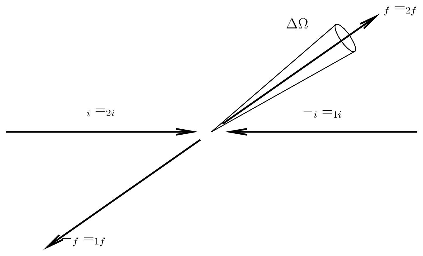
Figure 6:Two-body scattering as seen in the center-of-mass frame. Particle 2 comes in from the left, particle 1 from the right. The initial and final wave vectors of the two particles as seen in the center of mass frame are shown and expressed in terms of the initial and final wave vectors and of the center-of-mass motion.
Finally, to compute the differential cross we divide the differential transition rate by the incident flux, defined as as in Cross and Differential Cross In preparation for applications to scattering, we make a digression to define and discuss cross s and differential cross s. These concepts are best understood in a classical context, but most of the ideas carry over without trouble into quantum mechanics., where (one incident particle in the box of volume , where particle 2 can be thought of as the incident particle), and where is the relative velocity. Alternatively, we can think of two particles in a box of volume , so that , whereupon the integral in (62), taken over the box, gives . The conversion from transition rate to cross is the same in either case. The final differential cross is given by (86), with replaced by . As Figure 6 makes clear, the cross is measured in the center-of-mass frame.
All of this assumes that the two particles are distinguishable. If they are identical, then it is necessary to use properly symmetrized or antisymmetrized wave functions (including the spin), as discussed in 29. Identical Particles. See Prob.~\prbrtdpt-1. In this case one finds interference terms in the cross between the direct and exchanged matrix elements.
Another point of view is to include the center-of-mass dynamics in the description of the scattering process, that is, to use the entire Hamiltonian (93), including . In this case we take
The unperturbed eigenstates can be taken to be , with wave function
which are assumed to have periodic boundary conditions in a box of volume in both the coordinates and . The normalization is such that
where both the and integrations are taken over the volume , and the orthonormality relations are
The unperturbed energies are
The box is a mathematical crutch that allows us to deal with a discrete spectrum, and exactly how we set it up and the boundary conditions we impose are not important as long as gives physical results. In the present case, both and are quantized to lie on a lattice, as in (70). As , both and take on continuous values.
Now let be an initial state, and some final state. Given that commutes with the entire Hamiltonian , there cannot be any transitions that change the value of , so we must have if . This is true under the exact time evolution engendered by , and is not a conclusion of perturbation theory. However, we see the same thing in first order perturbation theory if we compute the matrix element of the perturbing Hamiltonian between the initial and final states,
where the -integration is the same as in (82). Except for the Kronecker delta in the total momentum, it is the same result obtained previously.
The Einstein frequency appearing in the expression for is
but, in view of the Kronecker delta in (101), the result is simply
for states for which does not vanish. This is just (72) all over again, with replaced by . The energy of the center-of-mass motion does not change in the scattering process.
Now squaring we get a probability of the transition in first-order, time-dependent perturbation theory, which we must sum over some collection of final states to get a physically meaningful result. Notice that the square of the Kronecker delta is just the same as the original Kronecker delta.
It is best to carry out the sum as follows. Let be a region of -space, which may or may not contain the initial momentum . Then we sum over all final in a cone as in Figs.~Figure 5 or Figure 6, and over all values in . Dividing the probability by the time , we interpret the result as the transition rate,
Here the 5 on indicates that is 3-dimensional and is 2-dimensional. (By the same logic we should write for the usual differential transition rate instead of , as we have been doing.) This integral can also be interpreted as
since the cone is small.
When we carry out the same sum on the probabilities, the Kronecker delta guarantees that the sum vanishes unless lies in the region . Finally, dividing by the incident flux , we can take the limit and the result is
This may be reinterpreted by writing
where the Dirac delta-function shows conservation of the center-of-mass momentum. Integrating this over all , we obtain
which reproduces our earlier results.
Application: Electrostatic Scattering and Form Factors
Let us consider the scattering of a charged particle by an electrostatic potential created by a charge distribution . The charge distribution need not be a point charge; for example, it could be the extended charge distribution inside a proton or a neutron (even though the neutron is neutral, it does contain a nontrivial charge distribution), or it could be the distribution created by the nucleus and the electron cloud of an atom. We denote the charge of the beam particle by .
The charge density and electrostatic potential are related by the Poisson equation,
and the potential appearing in the Schr"odinger equation is . The differential cross (86) requires the Fourier transform of , a useful expression for which can be obtained by Fourier transforming the Poisson equation. Denoting the variable upon which the Fourier transform depends by , as in (83), and noting that the operator in -space becomes multiplication by in -space, we find
where we use a tilde for the Fourier transforms of various quantities.
For use in the cross (86) we identify with the quantity
where now we write simply instead of for the final wave vector. Thus, the momentum transfer is
Then the cross (86) can be written
where
The quantity is called the form factor of the charge distribution; it is just the Fourier transform of , with a certain normalization.
We can transform the denominator in (113). Squaring (112), we have
where is the angle between the initial momentum and the final one , that is, it is the scattering angle; where we use , which is energy conservation; and where we use , where is the kinetic energy of the beam particle. Then the cross (113) becomes
Coulomb Scattering in the Born Approximation
Let us suppose the target is a point particle of charge , so that
Then
and (113) becomes
which we recognize as the Rutherford cross .
It is nice to derive the Rutherford cross by means of time-dependent perturbation theory, but the result is actually a fluke, for when we examine the conditions of validity of the approximations leading to (86) we find that in the case of the Coulomb potential they are not met for any value of the initial momentum. See \lippschw.7. This is a somewhat strange situation.
The Rutherford cross is exact for the classical scattering of two nonrelativistic, point charged particles in the electrostatic approximation (this is a standard calculation in classical mechanics). It turns out that it is also the exact cross for the Coulomb scattering of two distinguishable, nonrelativistic particles in the electrostatic approximation in quantum mechanics. This is shown by obtaining the exact solution of the Schr"odinger equation in the potential for positive energies and with the right boundary conditions. That is, the exact cross is obtained from exact solutions of the hydrogen-like Hamiltonian for positive energies. Recall that in 17. Hydrogen and Hydrogen-Like Atoms{} on hydrogen-like atoms we only considered bound state solutions. The exact positive energy solutions are somewhat more technical to deal with than the bound state solutions, but scattering solutions can be obtained by separating the Schr"odinger equation in confocal parabolic coordinates. The details are given in many books, for example, Schiff.
The details of this calculation are useful in many applications, for example, the calculation of thermonuclear reaction rates inside stars. Although the temperatures inside stars are quite high by ordinary standards the nuclei are still essentially nonrelativistic and ordinary Rutherford scattering applies to their interactions. A nuclear reaction requires that nuclei, which have positive charges and which therefore repel one another, come within the range of the nuclear forces. If the nuclei were governed strictly by classical mechanics they would never do this, since at the temperatures prevalent they do not have enough kinetic energy to overcome the repulsive Coulomb barrier. But a quantum treatment shows that there is some amplitude to tunnel through the barrier and bring the nuclei into contact, where the nuclear reactions can take place. Tunneling amplitudes have a strong dependence on energy (see Prob.~\wkb.3 for a one-dimensional example), which implies that thermonuclear reaction rates in stars are a strong function of temperature. The details are obtained from the exact scattering solution in the Coulomb potential.
When we use the Coulomb charge density (117) in the cross (116) we are effectively applying time-dependent perturbation theory to scattering in a hydrogen-like system, but we are only carrying the perturbation expansion out to lowest order in powers of the potential. Why then do we get the exact answer? Does it mean that all the higher order terms vanish?
The answer is more complicated than it seems, and must be understood in terms of the scattering amplitude, which is introduced in 36. Introduction to Time-Independent Scattering Theory and Scattering from Central Force Potentials. The cross is the square of the scattering amplitude, which is a complex quantity. It turns out that in the first Born approximation, equivalent to first-order time-dependent perturbation theory, the phase of the scattering amplitude for Coulomb scattering is completely wrong but by a kind of accident its absolute value is exactly right. Thus when we square the amplitude to get the cross , the phase cancels and we get the exact answer.
In the Coulomb scattering of identical particles, however, there are cross-terms between the direct and exchange amplitudes, needed to satisfy the symmetrization postulate, and these do depend on the phase of the scattering amplitude. Thus, the first Born approximation for the Coulomb scattering of identical particles does not give the right answer, since the cross terms are all wrong. See Prob.~\prbrtdpt-1.
Other Types of Electrostatic Scattering
All this does not mean that our result (113) or (116) is useless, however. The problem with the Coulomb potential, from the standpoint of time-dependent perturbation theory or the Born approximation, is that it has effectively an infinite range. The long-range nature of this potential shows up in the Rutherford cross by the fact that the cross diverges rather badly at , that is, it goes as . In the Coulomb potential there is a large probability of small-angle scattering, which obviously comes (speaking classically) from particles with a large impact parameter. Since the potential is long-range, these particles feel the Coulomb force and undergo some scattering.
On the other hand, we see from (113) that the form factor squared is a kind of fudge factor that converts the Rutherford cross into the actual cross for a distributed charge distribution . If the form factor should vanish at , that is, if its Taylor series should start with a term proportional to , then will cancel two of the powers of seen in the denominator in (113), so the cross will only diverge as at small angles, instead of . It turns out that the condition is equivalent to the vanishing of the total charge in (see Prob.~\prbrtdpt-3), which means that the charge distribution does not have a monopole moment. Then the potential does not have a Coulomb tail at large distances, rather it falls off as or faster, and much of the small-angle scattering present in the Rutherford cross is eliminated.
If in addition the target charge distribution has no electric dipole moment, then it turns out that is quadratic in for small values of , so that the denominator in the Rutherford cross is completely eliminated and the cross (113) is nonsingular at . In cases like this the conditions of validity of cross (113) are met for some initial momenta (basically, for high enough initial energy).
Consider, for example, the elastic scattering of electrons by a hydrogen atom. We model the atom as charge distribution described by a point nucleus and an electron cloud with charge density
where we use (29) and where we work in atomic units (). Adding the charge density of the nucleus to this and computing the Fourier transform, we obtain the form factor as
When this is used in (113) we obtain a cross for electron-hydrogen scattering that is useful at moderately high electron energies (by atomic standards, that is, or in atomic units).
The scattering of charged particles by atoms is important in calculating , the rate at which a charged particle loses energy per unit distance when passing through matter. This is an important problem in many areas such as experimental high energy physics. In practice the calculations often must be relativistic and must take into account both elastic and inelastic scattering. At sufficiently high energies, the energy loss for electrons and muons is dominated by bremsstrahlung, the emission of photons as the electron or muon is accelerated in the field of the atomic nucleus.
Experimental probes of the internal structure of the proton and neutron by electron scattering played an important role in showing that these particles are made up of three constituent point particles, now known as quarks. These experiments were carried out during the 1960’s at the Stanford Linear Accelerator, and many similar experiments, using a variety of incident particles and a variety of targets, have been performed since, accumulating a body of experimental evidence that has guided and confirmed the theory of quantum chromodynamics, the theory of the strong interactions. In these experiments the beam particles are relativistic, so that magnetic effects are important in addition to electric effects. As a result the relativistic treatment of the scattering requires more than one form factor, but the basic ideas are the same as in the nonrelativistic electrostatic model considered here.
Example: The Yukawa Potential
Simple models of nuclear interactions between nucleons such as the proton and neutron often make use of the Yukawa potential,
where and are constants. The Yukawa potential is obviously a kind of modified Coulomb potential, with the extra factor that cuts off the potential at a distance of the order of and gives it a finite range. In Yukawa’s day it was known that the nuclear forces have a finite range on the order of , and he was thinking of a generalization of electromagnetic forces that would incorporate this fact.
To use the Yukawa potential in (86) it is necessary to know its Fourier transform. The Fourier integral can be carried out directly by means of contour integration, but the following approach is easier. First we note that
an obvious generalization of the Poisson equation for a point charge in electrostatics, which can be derived by directly applying (23) and using . (123) shows that the Yukawa potential is the Green’s function of static solutions of the Klein-Gordon equation,
which is the simplest relativistic wave equation for a particle of mass , where
See 45. Introduction to Relativistic Quantum Mechanics and the Klein-Gordon Equation{} for more details. Note that where is the Compton wave length of the particle of mass appearing in the Klein-Gordon equation. See \finestruc.5 for an explanation of the physical meaning of the Compton wavelength.
In Yukawa’s application the numbers come out about right if the particle is identified with the -meson, whose mass is . This corresponds to a Compton wave length of
close to the known range of the nuclear forces. (In Yukawa’s day, however, there was some confusion between the -meson and what is now called the muon, as the muon was detected first and has a similar mass.) Yukawa’s idea was that the meson whose mass appears in his potential through was the boson that carries the strong interactions, in the same way as the photon carries the electromagnetic interactions. Note that the Klein-Gordon equation goes over to the usual wave equation as ; the latter of course comes out of Maxwell’s equations. In the same limit, the Yukawa potential becomes the Coulomb potential.
Now multiplying (123) by and Fourier transforming, we obtain
using our normalization conventions for the Fourier transform and as the variable conjugate to . From this and (128) we obtain the cross for scattering from a Yukawa potential,
This result depends on several parameters (, , and ), and it is valid only for certain ranges of them. The details can be worked out by the method of \lippschw.7.
If we set and take the limit , the Yukawa cross (128) goes over to the Rutherford cross . As discussed in Coulomb Scattering in the Born Approximation, however, this cannot be regarded as a valid derivation of the Rutherford cross .
Other Applications
Here are some other applications of time-dependent perturbation theory that we will consider later in the course. As an example of an atom interacting with a classical light wave, we shall study the photoelectric effect in 35. The Photoelectric Effect. In the photoelectric effect, a high energy photon, described by a classical light wave, ejects an electron from an atom, leaving behind a positive ion. Later we will consider the emission and absorption of radiation by an atom using the quantized theory of the electromagnetic field, that is, we will study the emission and absorption of photons. A similar example, one that requires second-order time-dependent perturbation theory, is the scattering of photons by matter. Later still we will consider a variety of relativistic processes that are applications of time-dependent perturbation theory, including relativistic scattering of charged particles and the creation and annihilation of electron-positron pairs.
Problems
Problem 1.
Some questions involving the scattering of identical particles.
(a) In classical mechanics we can always distinguish particles by placing little spots of paint on them. Suppose we have two particles in classical mechanics that are identical apart from insignificant spots of blue and green paint. (The spots have no effect on the scattering.) Suppose the differential cross in the center-of-mass system for the detection of blue particles is . What is the differential cross for the detection of particles when we don’t care about the color?
(b) Consider the scattering of two identical particles of spin in quantum mechanics. Work in the center-of-mass system, and let be the reduced mass. Consider in particular three cases: , , and . Organize the eigenstates of as tensor products of spatial states times spin states; make the spin states eigenstates of and , where , and make the spatial states properly symmetrized or antisymmetrized plane waves. Let the initial spin state be and the final one be . Since potential scattering cannot flip the spin, the cross will be proportional to . Find the differential cross in terms of
where is defined as in (83). Use the fact that to simplify the result as much as possible. Use notation like that in (86).
(c) For the three cases , , , assume that the initial state is unpolarized and that we do not care about the final spin state. Find the differential cross in terms of the quantities , , and .
(d) Work out the answer for the case of Coulomb scattering of two electrons, and compare to the classical Rutherford formula, (119). Express your answer in a notation similar to that of (119). The cross term you get in applying the results of part (c) to Coulomb scattering is actually incorrect; the trouble is that plane waves do not adequately represent the unbound Coulomb wave functions, which have long range, logarithmic phase shifts. The correct answer is called the Mott cross , which we will discuss later in class.
Although the result obtained in this problem for Coulomb scattering is not correct, the calculation does show that in the case of identical particles the cross involves interference terms between direct and exchange amplitudes. Also, there are other problems, for example, the scattering of two neutrons or two identical atoms, for which the technique gives answers that are correct in the appropriate range of parameters.
Problem 2.
A basic rule of nonrelativistic interactions is that electrostatic forces cannot flip spins. The reason is that spins respond to magnetic fields, not electric fields. The cross section (\eqr\cn.80) applies to a charged particle scattered by an electrostatic potential, and in the derivation we assumed that the particle was spinless. But if we had taken spin into account we would have reached the conclusion that the cross section is the same as (\eqr\cn.80) as long as the final spin state is the same as the initial spin state; and the cross section for flipping the spin is zero. This is under the assumption that the perturbing Hamiltonian is the potential .
If we take into account relativistic corrections, however, then there is a small probability for flipping the spin.
Consider the scattering of an electron by a central force potential . Suppose the electron spin of the incident beam is polarized in the direction. Including the spin-orbit interaction (13), find the differential cross for electrons polarized in the direction after the scattering. Express it as a certain factor times the cross (86). Notice that in (13) is called in these notes.
Note: It is common in scattering problems to assume that the incident particles are directed in the -direction. We do not want to do that in this problem, since the -direction is the direction of polarization of the spin of the incident electrons. Call the incident wave vector and the final one or just , as in these notes. These can be in any direction. Also note the identity (23).
This problem gives an example of inelastic scattering, in which the internal state of the particles can change as a result of the scattering, or perhaps new particles created. In this case it is the spin state of the incident particle that can change. Other examples include the scattering of an electron from an atom, in which the state of the atom may change, or scattering in which a photon is emitted, etc. In general, the different processes (elastic and inelastic) are called channels. High energy processes tend to have many inelastic channels.
Problem 3.
The that appears in the denominator of the Rutherford cross section (\eqr\cn.113) means that there is a large cross section for scattering by small angles, where the momentum transfer is small. Speaking classically, this is obviously due to the small angle scattering that particles experience at large impact parameters. Since the Coulomb potential dies off only slowly with distance, there is still significant scattering even at large impact parameters.
Let the electrostatic potential of the scatterer be , as in Application: Electrostatic Scattering and Form Factors. If we wish the form factor to suppress the small angle scattering, then we should require that at . Show that this implies that the total charge in the distribution vanishes. This makes sense: if the total charge vanishes, then at large distances there is no Coulomb tail to .
The form factor can be expanded in powers of for small ,
Show that if the source distribution has no electric dipole moment, then the first order term (proportional to ) vanishes. If the total charge is also zero, then the differential cross (86) does not diverge at . In particular, this is true for any rotationally symmetric charge distribution of zero total charge, like that of the hydrogen atom with the form factor (121).