15. Orbital Angular Momentum and Spherical Harmonics
Introduction
In 13. Representations of the Angular Momentum Operators and Rotations, we worked out the general theory of the representations of the angular momentum operators and the corresponding rotation operators. That theory made no assumptions about the kind of system upon which the angular momentum and rotation operators act, for example, whether it is a spin system or has spatial degrees of freedom, whether single particle or multiparticle, whether nonrelativistic or relativistic, etc., because most of the theory of rotations is independent of those details. We did work through the specific case of spin- systems in detail in 12. Rotations in Quantum Mechanics, and Rotations of Spin-1/2 Systems. In this set of notes we consider another important example of the theory of rotations, namely, a system consisting of a single particle moving in three-dimensional space. We assume either that the particle is spinless, or that the spin degrees of freedom can be ignored.
For most of these notes we make no assumptions about the Hamiltonian governing the single particle, but the theory of rotations is most useful in the case that the particle is moving in a central force field, that is, one for which the potential is a function of the radius only. We will discuss central force problems in 16. Central Force Motion.
In these notes we follow the usual custom in the physics literature of denoting the orbital angular momentum by instead of the general notation used earlier. Similarly, we use the quantum number instead of .
Rotation Operators for Spatial Degrees of Freedom
The wave function for a spinless particle in three dimensions can be written
where is the state vector and are the position eigenkets. The general relation of such wave functions to the measurement postulates was laid out in 04. Spatial Degrees of Freedom; in particular, we are assuming that the three components of the position vector by themselves form a complete set of commuting observables, so that the position eigenkets form a continuous basis for the Hilbert space of physical states.
Introductory courses on quantum mechanics usually define the orbital angular momentum of a single particle as . This formula is borrowed from classical mechanics, where is (usually, not always) the angular momentum of a single particle moving in three-dimensional space. In this course, however, angular momentum is defined as the generator of rotations, as explained in 12. Rotations in Quantum Mechanics, and Rotations of Spin-1/2 Systems\ and \repsamos. Therefore we begin with a definition of rotation operators on our single particle system, and then derive their generators.
Let us recall that we defined translation operators by
where is a displacement vector. This is (21). This definition makes sense, because if the particle is known to lie in a small region around position , then the translated quantum state must mean the particle is known to lie in a small region around . This is just what we mean by the active point of view in applying translations.
Similarly, let be a proper rotation, and define an operator by
This definition is physically reasonable, because the position eigenket is the state of the system after a measurement of the position operator has yielded the value , while is the state after such a measurement has given the value . For example, position can be measured by passing particle through a small hole in a screen, and if we rotate the screen so that the hole moves from to , then it is logical to call the state produced by the rotated measuring apparatus the rotated state.
This argument does not specify the phase of the rotated state, however, and if we were to worry about this we would insert a phase factor on the right hand side of (3) that would depend on both and . Similar concerns could also be raised when defining the translation operators. We will ignore this possible complication as it turns out to be unnecessary in kinetic-plus-potential problems, and we will just work with the definition (3). Problems with magnetic fields, however, force us to think about those phase factors more carefully. This could be foreseen by the fact that a gauge transformation, insofar as its effect on wave functions is concerned, is equivalent to a change in the phase conventions for the position eigenkets.
The definition (3) of the rotation operators is provisional until we have demonstrated several things. First, we note that (3) actually does specify the operator , because it gives the action of that operator on a set of basis vectors. By linearity, the action of on an arbitrary vector is thereby specified. Next, we note that the definition implies that forms a representation of the rotation group , that is,
This follows directly from the definition, since
(4) also implies
and
Next we work out the effect of on a wave function. We start with
expanding an arbitrary state in terms of the position eigenbasis. Next we apply to both sides, writing
for the rotated state. This gives
We now change variables in the integral, writing , so that
since . Thus we find
where we have dropped the prime on the dummy variable of integration.
We see that the wave function of the rotated state is given by
where we use the notation to mean the wave function of the rotated state . This may be compared to the corresponding formula in the case of translations,
which is a 3-dimensional version of (24). In both Eqs~(13) and (14), the transformed wave function, evaluated at some point, is the original wave function evaluated at the inverse transformed point. As explained in Translation Operators, a mnemonic for remembering this is to write for the “old” and “new” points and , respectively, and then to say, the value of the old wave function at the old point is equal to the value of the new wave function at the new point, that is,
This rule is necessary in the active point of view. For example, if the old wave function has a large concentration of probability around a point , then the new, rotated wave function must have a large concentration around the actively rotated point . See Fig.~\figr\spatialdof.1 for an illustration in the case of translations.
It is now easy to show that the operators are unitary. We simply compute the square norm of the new wave function,
where in the last step we have performed a change of variables of integration, , and then dropped the prime. We see that the norm of an arbitrary state is preserved by , which is therefore unitary. See Prob. Paragraph(c) and (d).
In summary, we have found a representation of the classical rotations acting on the Hilbert space of our quantum mechanical system by means of unitary operators. This is precisely the starting point for the theory laid out in 13. Representations of the Angular Momentum Operators and Rotations. Notice by the way that the representation is single-valued, that is, there is only one unitary operator for each . This means that of the possible values for the angular momentum quantum number shown in (33), the half-integer values cannot occur, since they lead to double-valued representations. That is, can only take on the values .
The Orbital Angular Momentum 
We define the orbital angular momentum as the generators of our rotation operators . We can find explicitly by working with infinitesimal rotations. Let us write such a rotation in axis-angle form,
where . The corresponding unitary operator is
which is the definition of . See (2) and (3).
We substitute these infinitesimal rotations into (13). On the right we will need , which is given by
that is, (17) with . Then (13) becomes
where we have expanded the right hand side out to first order in . The leading order terms cancel, and cancels from the first order terms, which can be written as
where we have introduced the momentum operator which is when acting on wave functions . Since and are arbitrary, (21) implies
Our definition (3) of the rotation operators gives a definition of angular momentum that coincides with the usual definition of orbital angular momentum in quantum mechanics.
According to the theory presented in 12. Rotations in Quantum Mechanics, and Rotations of Spin-1/2 Systems\ and \repsamos, the components of must satisfy the commutation relations,
That they do so is easily verified from the definition (22) (if it were not true, there would be something seriously wrong with the whole theory.) Next, following the theory laid out in 13. Representations of the Angular Momentum Operators and Rotations, we work on constructing the standard angular momentum basis.
Orbital Angular Momentum Operators in Spherical Coordinates
The standard angular momentum basis is an eigenbasis of the operators , with certain phase and other conventions. Thus in the present case the basis vectors are wave functions indexed by and such that
The key to finding these wave functions is to first find the “stretched” states, that is, the states with (the maximum value of for a given ). States for other values of can then be generated by applying lowering operators. The stretched wave functions satisfy (24) with . The operator is, however, somewhat difficult to work with. It turns out to be easier to specify the stretched state as the eigenstate of with eigenvalue which is annihilated by the raising operator. See (29). Thus the stretched state satisfies
These equations are most conveniently solved in spherical coordinates.
Writing out the three components of as differential operators in rectangular coordinates, we can apply the chain rule to transform them to spherical coordinates. The transformation is straightforward but requires some algebra. See the Jacobian matrices (24) and (25). The results are
The component is particularly simple in spherical coordinates, and it is not hard to see why: is the generator of rotations about the -axis, and is the azimuthal angle. The usual spherical coordinate system singles out the -axis for special treatment, which is why the operators and are more complicated.
Next we compute the raising and lowering operators,
and the Casimir operator ,
At this point we notice the relation of to the Laplacian operator,
See (23). We will come back to this formula later, but for now we are more interested in angular momentum than kinetic energy.
A striking feature about the operators in spherical components is that the radial differential operator does not occur in them (hence it does not occur in any function of , either, such as , , or the rotation operators ). The geometrical reason is that rotations in physical space change the direction of vectors, but not their magnitude; therefore the motion of the tip of a given vector takes place on the surface of a sphere. This is also true of infinitesimal rotations, which connect nearby points of the same value but different and values. Therefore the components of , in terms of which infinitesimal rotations are expressed, do not involve any differentiation with respect to .
The Hilbert Space of Wave Functions on a Sphere
Because of this fact, we can think of the angular momentum operators as acting on functions defined on the sphere, rather than on functions defined in the full 3-dimensional space. The radius of the sphere is unimportant (since when using it we are only interested the angular dependence), so we can take it to be a sphere of unit radius. This is often a useful point of view, and we will now make a small digression for notation for functions defined on the unit sphere.
We denote a point on the unit sphere either by or by , indicating a unit vector based at the origin whose tip lies on the unit sphere. For example, we will write . We will adopt a Dirac bra-ket notation for functions on the unit sphere, for example, making the association,
We define the scalar product of two such functions by
where . This makes the space of normalizable wave functions on the unit sphere into a Hilbert space. We define a -function on the unit sphere by
which is a function concentrated at the point . Then
for any function . We associate this -function with a ket by
where . Then we have
The Standard Angular Momentum Basis for Orbital Angular Momentum
We return to (25) and (26) for the stretched wave function , which we express in spherical coordinates. First, the equation (25) can be written,
which has the general solution
where is an arbitrary function. By the theory of 13. Representations of the Angular Momentum Operators and Rotations\ we know that must be a nonnegative integer or half-integer, but in fact (38) shows that must be an integer since otherwise the wave function would not be single-valued. Wave functions in quantum mechanics are single-valued functions of position because is just the expansion of the state with respect to the position eigenbasis, and the basis kets are single-valued. This is the same conclusion we reached earlier at the end of Rotation Operators for Spatial Degrees of Freedom. Thus we have determined the -dependence of the function .
To get the -dependence, we call on the -equation (26), using (28) for in spherical coordinates. Applying this to the form (38) for , the -derivatives can be carried out, whereupon we find
or, canceling various factors,
This has the solution,
where is an arbitrary function of , or
These are the stretched wave functions.
We see that the simultaneous eigenfunctions of and are indeed degenerate, since any radial function may appear in (42). In order to resolve these degeneracies, we may introduce an arbitrarily chosen basis of radial wave functions, and write
The index we use here serves the same purpose as the index used in 13. Representations of the Angular Momentum Operators and Rotations; it labels an arbitrarily chosen orthonormal basis in the stretched eigenspace. We see that the multiplicity of the integral values of on the Hilbert space of wave function is infinity.
Another approach is simply to throw away the radial variables, and work on the unit sphere. On the Hilbert space of wave functions on the unit sphere, the simultaneous stretched eigenfunction of and is
and it is nondegenerate. Therefore, on this Hilbert space, the multiplicity is zero for half-integral , and unity for integral . When we normalize using the rule
we find
where we have identified the normalized with the stretched spherical harmonic , and where we have introduced the conventional phase factor . Recall that in the general theory developed in 13. Representations of the Angular Momentum Operators and Rotations, the phase of the stretched state was left arbitrary.
To obtain the states corresponding to other values of , we can apply lowering operators. We use (44), making the replacements, , . By induction one can show that
and altogether we find
This formula is valid for all in the range, .
(48) can be expressed in terms of Legendre polynomials and associated Legendre functions. First we consider the case , and call on the Rodriguez formula for the Legendre polynomial [see Abramowitz and Stegun, Eq.~(8.6.18)],
where we set
Then (48) becomes
The choice of the phase factor in (46) was designed to make real and positive at the north pole (); this follows from (76).
Now let us consider the case . We can construct the for this case by applying raising operators to the state . Using induction on (49), we obtain
(This formula only works for integer angular momentum, since the value is possible only in this case.) Next we use induction to obtain
where we have introduced the associated Legendre function, defined by
[See Abramowitz and Stegun, Eq.~(8.6.6), and beware of the difference between their function and , see the on notation on p.~332.] Altogether, for we have
For the case , we go back to (48), we set , and we use (49) and (55). The result is
which is equivalent to
valid for any value of .
In summary, the standard angular momentum basis for the space of wave functions defined on the unit sphere consists of the 's. The irreducible subspaces are the -dimensional spaces of wave functions spanned by the 's for fixed with . There is precisely one such subspace for each integer value of in the Hilbert space of wave functions on the sphere. For the Hilbert space of wave functions on three-dimensional space, there is an infinite set of irreducible subspaces for each integer value of , that is, the spaces of wave functions spanned by for fixed and .
Notice that the theory of the 's is completely founded on the general theory of raising and lowering operators as laid out in 13. Representations of the Angular Momentum Operators and Rotations, and that even the phase conventions are the standard ones presented in those notes. Only the phase of the stretched state in (46) goes beyond the conventions established in those notes.
Table of 's
We present a short table of 's:
's in Cartesian Coordinates
Sometimes versions of the spherical harmonics in Cartesian coordinates are useful. If we multiply (46) by , we obtain
This is a homogeneous polynomial in , and of degree . We can create the 's for other values of by applying the lowering operator , which in Cartesian coordinates is
While carrying out the derivatives might be complicated, notice that each derivative , , , lowers the degree of the polynomial, while the multiplication by , or raises it back. Thus we see that , when expressed in Cartesian coordinates, is a homogeneous polynomial in , , and of degree , for all .
An important application of this fact is that under parity, which causes to go into , the function changes by . This is the parity of , and hence of the wavefunctions that occur in central force problems. Notice that the parity depends only on , and is independent of . Parity is covered in detail in 21. Parity.
Rotating 's
There are several interesting and useful results that follow from applying rotation operators to the 's. It is often important to rotate the 's, because by the very definition of the spherical coordinates , a privileged role has been assigned to the -axis. In addition, the -axis has been selected out again for a privileged role by the standard convention of working with eigenfunctions of and . In many problems it is necessary to refer calculations to another axis, something that can be done with rotation operators.
First let us write the ket to stand for the function , regarded as a function defined on the unit sphere, so that
Since we have determined that is the nondegenerate eigenfunction of and on the unit sphere, we do not need any extra quantum numbers in . We now apply a rotation operator specified by to a and use (13). We have
where in effect we rotate the in two ways, once by rotating the argument in three-dimensional space, and the other time by rotating it as a basis function in its irreducible subspace of Hilbert space. The matrix element in the final expression is a matrix, so we obtain
This may be recognized as a special case of (91).
(64) gives at one point on the sphere as a linear combination of other 's, for the same value of but all values of , at another point on the sphere. The fact that the linear combination does not involve other values of is due to the invariance of the irreducible subspace spanned by the 's for fixed but variable , under the action of rotations.
(64) can be used to express the values of the 's at a point of interest in terms of the their values at the north pole (a convenient reference point). To put this in convenient form, we change notation in (64), and replace by , and replace by . Then we write , so that is interpreted as a rotation that maps the -axis into some direction of interest. Then we obtain
If we write for the direction of interest, then a rotation that maps the -axis into this direction is easily given in Euler angle form,
that is, with and , because the first two Euler angles were designed to specify the direction of the rotated -axis. Also, the value of at the north pole is especially simple, because all the associated Legendre functions vanish at unless , and in that case we have . Therefore
Finally, we can use (73) to rewrite the matrix , and (65) becomes,
In this way we have found a useful connection between the 's and the -matrices.
The Addition Theorem for Spherical Harmonics
We can use this to derive another nice result. Consider the following function defined on the unit sphere:
where is the usual Legendre polynomial and is some direction of interest. Now let us rotate this function by some rotation specified by . We have
where in the final step we use the fact that to transfer the rotation matrix from to in the scalar product. See Prob. Paragraph(a). Now we choose the matrix to have the Euler angle form , so that , where is another direction of interest (in addition to ). Then (69) and (70) become
where we use (64) to expand the rotated . Finally, we use (68) to write the result purely in terms of 's, and we have
which is the (very useful) addition theorem for the spherical harmonics.
The Multipole Expansion in Electrostatics
We will now review the multipole expansion in electrostatics, which fits in well at this point in the presentation and which will be of use several times in the course.
We begin with the Legendre polynomials, which are defined by
where the series converges for . That is, they are the coefficients of the expansion of the left-hand side in powers of the parameter . The left-hand side is considered the generating function of the Legendre polynomials. Carrying out the expansion, we find the first few Legendre polynomials,
Note that if we set in (73) we obtain
Comparing the Taylor series expansion of the left-hand side with the series on the right, we find
This is essentially the standard normalization for the Legendre polynomials.
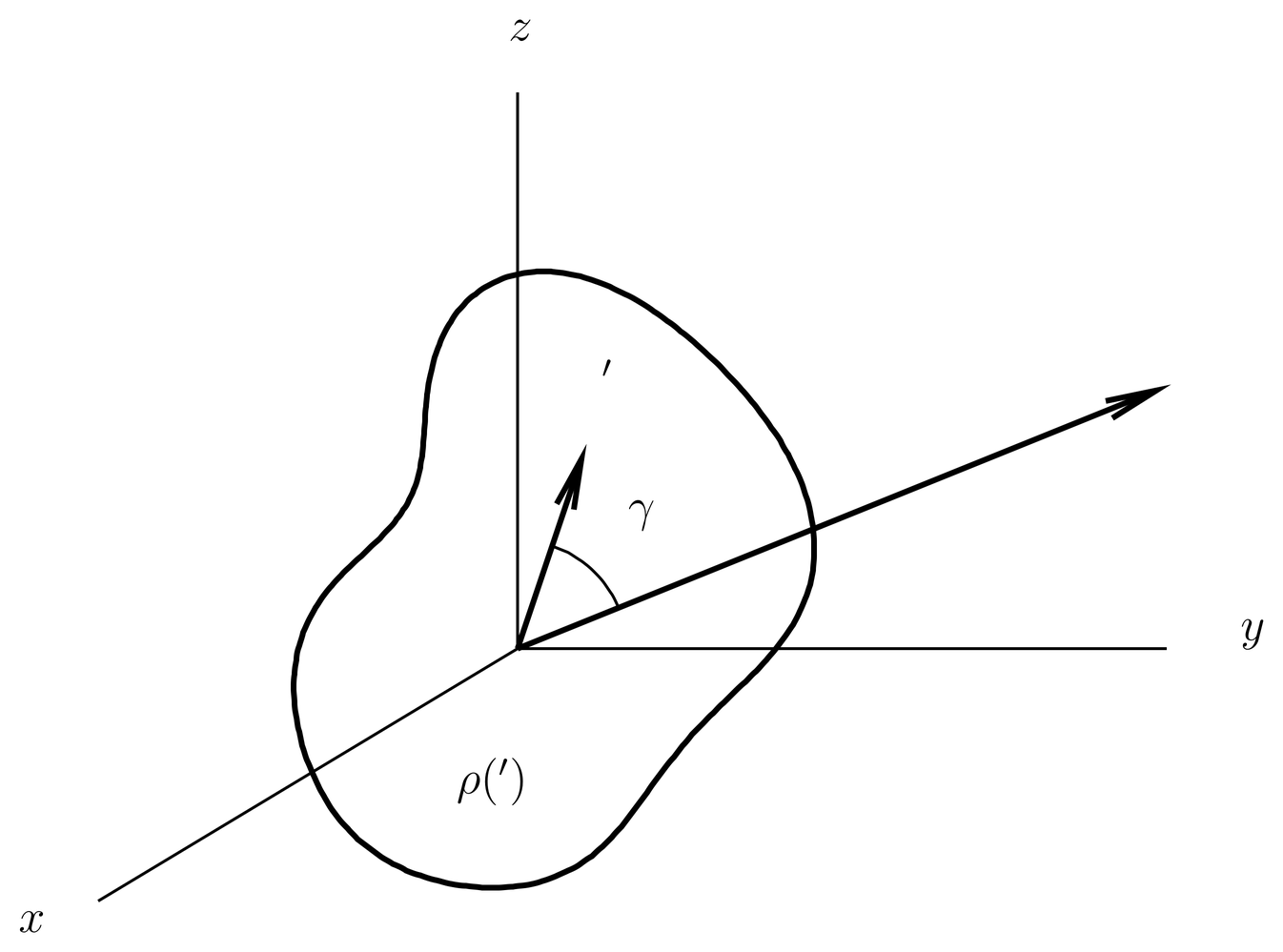
Figure 1:The origin of a system of coordinates is located inside a localized charge distribution with density . The variable runs over the charge distribution, while is a field point at which the potential is desired.
Now consider a localized charge distribution , as in Figure 1, with a field point that is well outside the distribution. The electrostatic potential at is given by
[see (5)], where the variable of integration runs over the charge distribution. Writing and , we have
where and is the angle between the vectors and , as shown in the figure. Then using the expansion (73) we have
where in the last step we use the addition theorem (72), and where are the spherical coordinates of and are those of . This allows us to write the potential as
where the coefficients characterize the charge distribution and are given by
Since is a homogeneous polynomial in of degree (see 's in Cartesian Coordinates), the coefficients are moments of degree of the charge distribution. (80) is the multipole expansion of the potential in spherical coordinates. The terms fall off with distance as , so that at large distances the first nonvanishing term dominates.
The multipole expansion in rectangular coordinates is also useful. Expanding directly in powers of , assuming , we obtain
We substitute this into (77) and write the potential in terms of the contributions at various orders by . At order we have
where is the zeroth moment of the charge distribution, that is, it is the total charge,
At order we obtain
where is the first moment of the charge distribution, that is, it is the dipole moment vector,
As for the term , we note first that the tensor which appears in (82) is symmetric and traceless, and that it is contracted against which is symmetric but not traceless. However, we can subtract the trace from without changing the result, since contracted against vanishes. This allows us to write the second order term in (82) more symmetrically as
Then the contribution to the potential can be written as
where is the quadrupole moment tensor,
Notice that is also symmetric and traceless. Equations~(83), (85) and (88) give the monopole, dipole and quadrupole contributions to the potential, respectively, in rectangular coordinates.
By comparing the monopole term in rectangular coordinates to that in spherical coordinates, we see that , since . The dipole and quadrupole terms will be compared in 20. The Wigner-Eckart Theorem.
Finally, we note that sometimes the field point is inside the charge distribution. In that case it is convenient break the region of integration into the region , where we expand in the ratio , and the region , where we expand in the ratio . The expansion is conveniently written as
where and .
Orbital Angular Momentum in Multiparticle Systems
Consider now a system of spinless particles moving in three-dimensional space. The basis kets are , and the wave functions are . The obvious generalization of the definition (3) of the rotation operators is
or, in wave function language,
as in (13). By considering infinitesimal rotations it is easy to work out the generator of rotations; it is
The orbital angular momentum for the entire system is the sum of the orbital angular momenta for the individual particles.
It may be of interest to rotate some of the particles and not others. For example, the operator that rotates only particle while leaving the others alone is
Such operators are useful when the system is invariant under rotations of the individual particles (for example, in the central field approximation in atomic physics).
The standard angular momentum basis for a multiparticle system is best constructed by means of coupling of angular momenta, a topic covered in 18. Coupling of Ket Spaces and the Addition of Angular Momenta.
Problems
Problem 1.
Consider wave functions on the unit sphere, as in Sec.~\secr\cn.5. Using the differential operators in Sec.~\secr\cn.4, find the simultaneous eigenfunction of and with eigenvalues and , respectively (that is, the case ). Normalize this wave function but leave leave a phase factor that will be determined later. Now apply twice to this state fill out the standard basis vectors in an irreducible subspace. The wave functions are proportional to for . By requiring to be real and positive at the north pole, determine the phase. Compare your answers to a table of 's. (See Sec.~\secr\cn.7.)
Problem 2.
Some problems concerning orbital angular momentum in the momentum representation.
(a) Consider a spinless particle moving in three-dimensional space. It was shown The Standard Angular Momentum Basis for Orbital Angular Momentum that the standard angular momentum basis consists of wavefunctions of the form }, where is an arbitrary basis of radial wave functions. The wave functions being referred to here are configuration space wave functions, or . Consider the wave functions in the momentum representation. Let be spherical coordinates in momentum space, that is,
Find the form of the wavefunctions that make up the standard angular momentum basis in momentum space.
(b) Let be a wave function in three dimensions, and let be the rotated wave function corresponding to rotation matrix . Use (13) and the usual expression for the momentum space wave function,
to find a relation between and .
(c) A useful formula in scattering theory is the expansion of a plane wave in terms of free particle solutions of definite angular momentum. It is
where is the angle between and , where is a spherical Bessel function, and where is a Legendre polynomial.
Suppose . Show that , and find a one-dimensional integral transform connecting the radial functions and .
Problem 3.
A problem on the addition theorem for spherical harmonics.
(a) Suppose unitary operators on some Hilbert space satisfy the representation property, (4). By taking matrix elements with respect to a standard angular momentum basis , translate that condition into an equivalent condition in terms of -matrices.
(b) Show that the addition theorem for spherical harmonics, (72), is a special case of the preceding result.