19. Transformation of Operators Under Rotations
Introduction
In both classical and quantum mechanics we classify observables according to how they transform under symmetries, including proper rotations, improper rotations, Lorentz transformations, etc. For example, we speak of scalars, vectors, tensors, pseudoscalars, pseudovectors, etc. In these notes we examine how operators transform under proper rotations, developing a classification scheme that will be important for understanding rotational symmetry in quantum mechanics. We will take up the case of improper rotations in 21. Parity, time reversal in 22. Time Reversal, and Lorentz transformations in 48. Covariance of the Dirac Equation. The material of these notes is background on the Wigner-Eckart theorem, which we take up in 20. The Wigner-Eckart Theorem.
Definition of a Rotated Operator
We consider a quantum mechanical system with a ket space upon which rotation operators , forming a representation of the classical rotation group , are defined. The representation will be double-valued if the angular momentum of the system is a half-integer. In these notes we consider only proper rotations ; improper rotations will be taken up later. The operators map kets into new or rotated kets,
where is the rotated ket. We will also write this as
In the case of half-integer angular momenta, the mapping above is only determined to within a sign by the classical rotation .
Now if is an operator, we define the rotated operator by requiring that the expectation value of the original operator with respect to the initial state be equal to the expectation value of the rotated operator with respect to the rotated state, that is,
which is to hold for all initial states . But this implies
or, since is arbitrary [see Prob. Paragraph(b)],
Solving for , this becomes
which is our definition of the rotated operator. We will also write this in the form,
Notice that in the case of half-integer angular momenta the rotated operator is specified by the rotation matrix alone, since the sign of cancels and the answer does not depend on which of the two rotation operators is used on the right hand side. This is unlike the case of rotating kets, where the sign does matter. (7) defines the action of rotations on operators.
Scalar Operators
Now we classify operators by how they transform under rotations. First we define a scalar operator to be an operator that is invariant under rotations, that is, that satisfies
for all operators . This terminology is obvious. Notice that it is equivalent to the statement that a scalar operator commutes with all rotations,
If an operator commutes with all rotations, then it commutes in particular with infinitesimal rotations, and hence with the generators . See (13). Conversely, if an operator commutes with (all three components), then it commutes with any function of , such as the rotation operators. Thus another equivalent definition of a scalar operator is one that satisfies
The most important example of a scalar operator is the Hamiltonian for an isolated system, not interacting with any external fields. The consequences of this for the eigenvalues and eigenstates of the Hamiltonian are discussed in Secs.~Energy Eigenstates in Isolated Systems and The Nucleus and the M"ossbauer Effect below.
Vector Operators
In ordinary vector analysis in three-dimensional Euclidean space, a vector is defined as a collection of three numbers that have certain transformation properties under rotations. It is not sufficient just to have a collection of three numbers; they must in addition transform properly. Similarly, in quantum mechanics, we define a vector operator as a vector of operators (that is, a set of three operators) with certain transformation properties under rotations.
Our requirement shall be that the expectation value of a vector operator, which is a vector of ordinary or -numbers, should transform as a vector in ordinary vector analysis. This means that if is a state and is the rotated state as in (1), then
which must hold if is to be considered a genuine vector operator. In case the notation in (11) is not clear, we write the same equation out in components,
(11) or (12) is to hold for all , so by (1) they imply
or, (after swapping and )
Inn components this is
We will take (13), (14) or (15) as the definition of a vector operator.
In the case of a scalar operator, we had one definition (8) involving its properties under conjugation by rotations, and another (10) involving its commutation relations with the angular momentum . The latter is in effect a version of the former, when the rotation is infinitesimal. Similarly, for vector operators there is a definition equivalent to (14) or (15) that involves commutation relations with . To derive it we let and in (14) have axis-angle form with an angle , so that
and
See (22) and (32) for the latter. Then the definition (14) becomes
or
Taking the -th component of this, we have
or, since is an arbitrary unit vector,
Any vector operator satisfies this commutation relation with the angular momentum of the system.
The converse is also true; if (21) is satisfied, then is a vector operator. This follows since (21) implies (19) which implies (18), that is, it implies that the definition (14) is satisfied for infinitesimal rotations. But it is easy to show that if (14) is true for two rotations and , then it is true for the product . Therefore, since finite rotations can be built up as the product of a large number of infinitesimal rotations (that is, as a limit), (21) implies (14) for all rotations. Equations (14) and (21) are equivalent ways of defining a vector operator.
We have now defined scalar and vector operators. Combining them, we can prove various theorems. For example, if and are vector operators, then is a scalar operator, and is a vector operator. This is of course just as in vector algebra, except that we must remember that operators do not commute, in general. For example, it is not generally true that , or that .
If we wish to show that an operator is a scalar, we can compute its commutation relations with the angular momentum, as in (10). However, it may be easier to consider what happens when the operator is conjugated by rotations. For example, the central force Hamiltonian (1) is a scalar because it is a function of the dot products and . See The Radial Schr"odinger Equation.
Examples of Vector Operators
Consider a system consisting of a single spinless particle moving in three-dimensional space, for which the wave functions are and the angular momentum is . To see whether is a vector operator (we expect it is), we compute the commutation relations with , finding,
According to (21), this confirms our expectation. Similarly, we find
so that is also a vector operator. Then (see transfop-4) must also be a vector operator, that is, we must have
This last equation is of course just the angular momentum commutation relations, but here with a new interpretation. More generally, by comparing the adjoint formula (95) with the commutation relations (21), we see that the angular momentum is always a vector operator.
If it Looks Like a Vector 
Not everything that looks like a vector is a vector operator, according to our definition (15). Consider, for example, the Stark effect, in which an atom interacts with an external electric field . If the atom has a single electron, then the interaction term in the Hamiltonian is the potential
The vector is a vector operator, as we have seen, but what about ? It is in fact just a vector of -numbers, which, regarded as multiplicative operators on wave functions, commute with everything. Therefore we have
which does not satisfy the definition (15) of a vector operator. Since is not a vector operator, is not a scalar operator.
To understand this situation, we note that the rotation operators rotate the physical observables of our system, such as the position and momentum of the electron. They do not rotate external parameters, such as . On the other hand, the external electric field is created by some charges somewhere. Imagine, for example, that the atom is between the plates of a capacitor, with charges arrayed along the plates to create . If these charges are included in “the system,” then when we rotate the system the field is rotated as well. Then becomes a vector operator and becomes a scalar operator.
We will see similar issues regarding the definition of “the system” when we come to conservation of parity and time reversal.
Tensor Operators
Finally we define a tensor operator as a tensor of operators with certain transformation properties that we will illustrate in the case of a rank-2 tensor. In this case we have a set of 9 operators , where , which can be thought of as a matrix of operators. These are required to transform under rotations according to
which is a generalization of (15) for vector operators. As with scalar and vector operators, a definition equivalent to (27) may be given that involves the commutation relations of with the components of angular momentum.
As an example of a tensor operator, let and be vector operators, and write
Then is a tensor operator (it is the tensor product of with ). This is just an example; in general, a tensor operator cannot be written as the product of two vector operators as in (28). In practice, however, many tensor operators appear as linear combinations of such products.
Consider, for example, the quadrupole moment operator. In a system with a collection of particles with positions and charges , where indexes the particles, the quadrupole moment operator is
This is obtained from (89) by setting
The quadrupole moment operator is especially important in nuclear physics, in which the particles are the protons in a nucleus with charge . Notice that the first term under the sum (29) is an operator of the form (28), with .
Tensor operators of other ranks (besides 2) are possible; a scalar is considered a tensor operator of rank 0, and a vector is considered a tensor of rank 1. In the case of tensors of arbitrary rank, the transformation law involves one copy of the matrix for each index of the tensor.
Invariant and Irreducible Subspaces of Operators
Let us return to (15), the transformation law defining a vector operator. This says that if we rotate any one of the components of a vector operator, we get a linear combination of the three components of that vector operator. The same is true if we rotate any linear combination of the three components.
In this respect it is useful to think of the space of operators as a vector space, and the components of a vector operator as “basis operators” that span a 3-dimensional subspace of the space of operators. (We assume the vector operator is not identically zero.) Operators form a vector space because they can be added to one another and multiplied by scalars, that is, linear combinations of operators are operators.
Then the 3-dimensional subspace of operators spanned by the components of a vector operator is invariant under the action of rotations, which is defined by (7). This means that if we rotate any operator belonging to this subspace, we obtain another operator belonging to the same subspace, a fact that is a simple consequence of (15).
Similarly, the nine components of a tensor operator, if linearly independent, span a 9-dimensional space of operators that according to the definition (27) is invariant under the action of rotations.
Another example of an invariant subspace of operators is the 1-dimensional subspace spanned by any nonzero scalar operator , as follows from the definition (8) of a scalar operator.
Thus, we have three examples of subspaces of operators that are invariant under rotations, those spanned by the components of a scalar operator, a vector operator, or a second-rank tensor operator, which are of dimensionality 1, 3 and 9 respectively.
Now in general when we have a subspace (of any vector space) that is invariant under rotations, we can ask if it possesses a smaller subspace that is also invariant. If it does, we say it is reducible; it not, it is irreducible. Invariant, reducible subspaces can always be broken up into smaller invariant, irreducible subspaces, so that the irreducible subspaces are the building blocks of reducible subspaces. It turns out that the invariant, irreducible subspaces are orthogonal to one another.
By our definition, every invariant, 1-dimensional subspace is automatically irreducible, because it contains no smaller subspace. Therefore the 1-dimensional subspace of operators spanned by a scalar operator is automatically irreducible.
What about the 3-dimensional subspace spanned by the components of any nonzero vector operator? It turns out that this, too, is irreducible. See Prob.~\prbrtransfop-2.
What about the 9-dimensional space spanned by the components of a tensor operator (we assume the nine components are linearly independent)? It turns out this subspace is reducible. To see how, let us work with the example (28) of a tensor operator, . We draw attention to the trace of this tensor,
which as shown is the dot product of the two vector operators and . This is a scalar, which is invariant under rotations, so the 9-dimensional space of operators spanned by the has a 1-dimensional, invariant subspace, spanned by . This subspace, being 1-dimensional, is irreducible.
This leaves a complementary, 8-dimensional subspace of operators. Is this reducible? Yes, it possesses a 3-dimensional invariant subspace spanned by the operators
or, in other words,
The components of form a vector operator, so by themselves they span an irreducible invariant subspace under rotations. As we see, the components of contain the antisymmetric part of the original tensor .
The remaining 5-dimensional subspace is irreducible. It is spanned by operators containing the symmetric part of the tensor , with the trace removed (or, as we say, the symmetric, traceless part of ). The following five operators form a basis in this subspace:
The original tensor breaks up in three irreducible subspaces, a 1-dimensional scalar (the trace), a 3-dimensional vector (the antisymmetric part), and the 5-dimensional symmetric, traceless part. Notice that these dimensionalities are in accordance with the Clebsch-Gordan decomposition,
which corresponds to the count of dimensionalities,
This Clebsch-Gordan series arises because the vector operators and form two irreducible subspaces of operators, and when we form according to , we are effectively combining angular momenta as indicated by (35). The only difference from our usual practice is that we are forming products of vector spaces of operators, instead of tensor products of ket spaces.
We have examined this decomposition in the special case , but the decomposition itself applies to any second rank tensor . More generally, Cartesian tensors of any rank are reducible.
It is possible that a given tensor may have one or more of the three irreducible components that vanish. The quadrupole moment tensor (29), for example, is already symmetric and traceless, so its nine components are actually linear combinations of just five linearly independent operators. For another example, an antisymmetric tensor satisfying contains only the three-dimensional (vector) subspace.
The decomposition of a tensor operator into its irreducible components gives us a preview of how angular momentum quantum numbers are attached to operators. This topic will be developed in more detail in 20. The Wigner-Eckart Theorem.
Energy Eigenstates in Isolated Systems
In this we explore the consequences of rotational invariance for the eigenstates, eigenvalues and degeneracies of a scalar operator. The most important scalar operator in practice is the Hamiltonian for an isolated system, so for concreteness we will speak of such a Hamiltonian, but the following analysis applies to any scalar operator.
Let be the Hamiltonian for an isolated system, and let be the Hilbert space upon which it acts. Since is a scalar it commutes with , and therefore with the commuting operators and . Let us denote the simultaneous eigenspaces of and with quantum numbers and by , as illustrated in Fig.~\figr\repsamos.5. It was shown in 13. Representations of the Angular Momentum Operators and Rotations{} that for a given system, takes on certain values that must be either integers or half-integers. For example, in central force motion we have only integer values of (which is called in that context), while for the nucleus, which is discussed in more detail in the next , we have only half-integer values. For each value of that occurs there is a collection of eigenspaces of and , for . These spaces are mapped invertibly into one another by and , as illustrated in Fig.~\figr\repsamos.5, and if they are finite-dimensional, then they all have the same dimension. As in 13. Representations of the Angular Momentum Operators and Rotations, we write , which we call the multiplicity of the given value.
In 13. Representations of the Angular Momentum Operators and Rotations{} we constructed a standard angular momentum basis by picking an arbitrary orthonormal basis in each stretched space , with the basis vectors labeled by as in Fig.~\figr\repsamos.5, where . We denote these basis vectors in by . Then by applying lowering operators, we construct an orthonormal basis in each of the other , for running down to . In this way we construct a standard angular momentum basis on the whole Hilbert space . In this construction, it does not matter how the basis is chosen in , as long as it is orthonormal.
Now, however, we have a Hamiltonian, and we would like a simultaneous eigenbasis of , and . To construct this we restrict to for some (see Simultaneous Eigenbases of Commuting Observables for the concept of the restriction of an operator to a subspace, and how it is used in proving that commuting operators possess a simultaneous eigenbasis). This restricted is a Hermitian operator on so it possesses an eigenbasis on that space.
The spectrum of on can be either discrete, continuous, or mixed (in most problems we will consider in this course it has a continuous spectrum above a threshold energy, and may have discrete bound states below that). Let us focus on the bound states and assume that possesses at least one bound eigenstate on with corresponding eigenvalue . Then satisfies
Now by applying a lowering operator we find
so that is an eigenstate of , lying in the space , with the same eigenvalue as . Continuing to apply lowering operators, we generate a set of linearly independent eigenstates of with the same eigenvalue , that is, is independent of the quantum number . These states span an irreducible, invariant subspace of .
There may be other irreducible subspaces with the same energy. This can occur in two ways. It could happen that there is another energy eigenstate in , linearly independent of , with the same energy . That is, it is possible that is a degenerate eigenvalue of restricted to . In general, every discrete eigenvalue of restricted to corresponds to an eigenspace, a subspace of that may be multidimensional. Choosing an orthonormal basis in this subspace and applying lowering operators, we obtain a set of orthogonal, irreducible subspaces of the same value of , each with dimensions and all having the same energy.
It could also happen that there is another bound energy eigenstate, in a different space for , with the same energy as . This would be a degeneracy of that crosses values. If such a degeneracy exists, then we have at least two irreducible subspaces of the same energy, one of dimension and the other of dimension . In other words, degeneracies can occur either within a given value or across values.
These facts that we have accumulated can be summarized by a theorem:
Let us look at two examples of how this theorem works out in practice, the first a simple one with a small number of degrees of freedom that is exactly solvable, and the other a complicated one with a large number of degrees of freedom, in which all we know about the Hamiltonian is that it is invariant under rotations.
Example: Central Force Motion
For the simple example we take the case of central force motion, for which we use the notation , etc.{} instead of , etc.
In central force motion the stretched subspace consists of wave functions , where is any radial wave function. To find the energy eigenstates in this stretched subspace we solve the radial Schr"odinger equation for the given value, which produces in general a continuous and a discrete spectrum. We assume there is a discrete spectrum for the given value and denote the energy eigenvalues and corresponding radial wave functions by and , as in 16. Central Force Motion. By applying lowering operators to the wave function , we obtain an irreducible subspace of degenerate energy eigenfunctions, spanned by .
Now we consider degeneracies. Is it possible, for a given value of in a central force problem, that a bound energy eigenvalue can be degenerate? That is, can there be more than one linearly independent bound energy eigenstate of a given energy in ? As discussed in Quantum Numbers and Degeneracies, the answer is no, the boundary conditions on the radial wave functions guarantee that there can be no degeneracy of this type. In central force problems, we do not have degeneracies within a given value.
Then is it possible that there is a degeneracy between different values of ? Again, as discussed in 16. Central Force Motion, the answer is that in general it is not very likely, since the different radial equations for different values of are effectively different Schr"odinger equations whose centrifugal potentials are different.
The fact is that systematic degeneracies require a symmetry. We are already taking into account the symmetry of proper rotations, which explains the degeneracy in the magnetic quantum number , so any additional degeneracy will require a larger symmetry group than . In the absence of such extra symmetry, degeneracies between different values can occur only by “accident,” that is, by fine tuning parameters in a Hamiltonian to force a degeneracy to happen. This is not likely in most practical situations. Therefore in central force problems we do not normally expect degeneracies that cross subspaces of different values of .
As explained in 17. Hydrogen and Hydrogen-Like Atoms, however, the electrostatic model of hydrogen is a notable exception, due to the symmetry group possessed by this model, which is larger than the rotation group . The extra symmetry in this model of hydrogen explains why the energy levels (in the right units) are the same across the angular momentum values . The isotropic harmonic oscillator in two or more dimensions is another example of a system with extra degeneracy; such oscillators are approximate models for certain types of molecular vibrations.
For a more complicated example of how Theorem~Theorem works out in practice we examine some energy levels of the nucleus , which is important in the M"ossbauer effect. We use the opportunity to digress into some of the interesting physics connected with this effect. We begin with a general discussion of aspects of the emission and absorption of photons by quantum systems.
Emission and Absorption of Photons
When an atom, nucleus or other quantum system is in an excited state and emits a photon while dropping into the ground state ,
then a simple description of the process says that the energy of the photon is given by
where and are the energies of the states and . If now there is another atom, nucleus or other system of the same type nearby in its ground state , then it would appear that that photon has exactly the right energy to induce the inverse reaction,
thereby lifting the second system into the excited state .
Does this mean, for example, that when an atom in a gas emits a photon that the photon only travels as far as the nearest neighboring atom before being absorbed again? No, because there are several effects that complicate the basic picture just presented, modifying the energy of the photon so that is it not exactly given by (40). These include the natural line width of the transition ; Doppler shifts; recoil; and, in the case of nuclei, what are called chemical shifts.
In quantum mechanics the energy of a system is only precisely defined in a process that takes place over an infinite amount of time. The excited state of our system is unstable with some lifetime , so its energy is only defined to within an uncertainty of order . Assuming is the ground state, it is stable and can exist over an infinite amount of time, so there is no uncertainty in its energy. Overall, the uncertainty in the energy creates uncertainty of order to the energy of the photon emitted in the process (39). This can be seen experimentally; if all other sources of broadening of the spectral line are eliminated, then the energy of photons emitted in an atomic or nuclear transition does not have a definite value, but rather there is a spread of order about the nominal value . This spread is called the natural line width of the spectral line. The natural line width of spectral lines is examined in some detail in 44. Natural Line Width, Long-Time Behavior and the Lamb Shift.
Similarly, if a photon of energy encounters a quantum system of the same type at rest in its ground state , then if is roughly within the range about the nominal energy it will be able to lift the second system into the excited state , that is, the inverse reaction (41) will take place.
On the other hand, if the emitting atom, nucleus or other quantum system is in a state of motion, then the frequency of the emitted photon will be Doppler shifted and may no longer be within the resonance needed to raise another such system into its excited state. Writing simply for the nominal energy of the photon, the velocity needed to shift the photon out of resonance is given by
Whether or not the photon is shifted out of resonance depends on the velocity and other parameters, but in many practical circumstances one will find that thermal velocities do exceed the value given by (42). A similar logic applies in case the receiving system is in a state of motion (or both, as would be the case of a gas).
Even if the emitting atom or nucleus or other system is at rest, the energy is not given exactly by (40) because of the recoil of the emitting system when the photon is emitted. The photon has energy and momentum where , so by conservation of momentum the emitting system suffers a recoil and has momentum after the photon of frequency is emitted, where is the mass of the emitting system. Thus (40) should be replaced by
where is the recoil velocity. Some of the available energy goes into kinetic energy of the recoiling system, and the energy of the emitted photon is actually less than the nominal value (40). Again, whether this recoil shift is greater or less than the natural line width depends on the parameters of the problem.
The Nucleus and the M"ossbauer Effect
The M"ossbauer effect involves a transition between two energy levels of the nucleus, where the simple notation (or ) refers to the ground state and (or ) refers to an excited state. These states are illustrated in the energy level diagram for the nucleus given in Figure 1. The photon emitted has energy 14.4~KeV, and the lifetime of the excited state is ~sec. From these figures we find , where and are the energy and frequency of the emitted photon. The spread in the energy is very small compared to the energy. For example, according to (42), to Doppler shift the photon out of resonance it would require a velocity of , or .
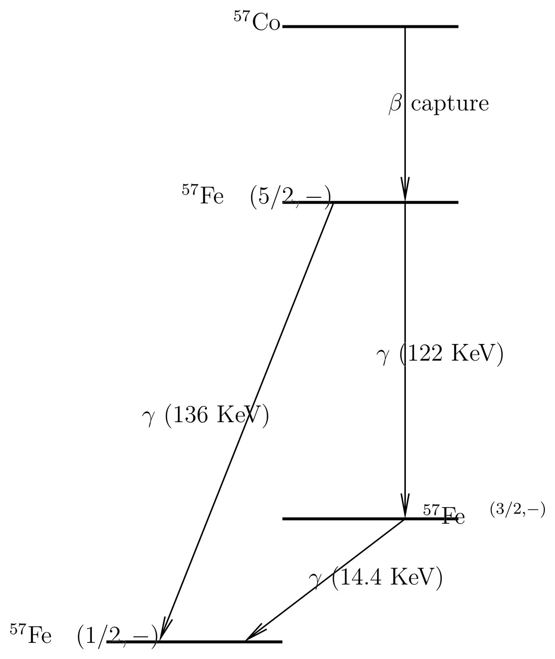
Figure 1:Energy level diagram relevant for the M"ossbauer effect in . is the ground state, is an excited state, and is a more highly excited state. Principal transitions via photon emission are shown.
The M"ossbauer effect makes use of a source containing iron nuclei in the excited state , which emits photons, and a receiver containing iron nuclei in the ground state which may absorb them by being lifted into the excited state via the reverse reaction. The receiver can be a block of natural iron, which contains the isotope at the 2% level, behind which a gamma-ray detector is placed. If the incident photons are within the narrow resonant range of energies, then they will be absorbed by the block of iron, and the detector will detect nothing. But if they are shifted out of resonance, the gamma rays will pass through the block of iron and the detector will detect them. If there is some effect that shifts the frequency of the gamma rays from their nominal energy (for example, the gravitational red shift in the Pound-Rebka experiment), then a compensating Doppler shift can be introduced by giving the source some velocity. By measuring the velocity of the source needed to shift the gamma rays back into resonance, one can measure the shift caused by the effect in question.
However, plugging in the numbers shows that the recoil shift described by (43), where is the mass of an iron nucleus, is much greater than the natural line width, so the recoil would seem to spoil the whole idea. But the iron nucleus is not free, rather it is part of a crystal lattice, whose vibrations are described by a large number of harmonic oscillators, the normal modes of the lattice. (See the discussion in Harmonic Oscillators in Mechanical Systems.) Thus the recoil kinetic energy in (43) is not free to take on any value, rather it must be some multiple of , where is the frequency of a normal mode of the lattice. That is, when the photon is emitted by the nucleus, some number of phonons are also emitted into the lattice, representing the recoil energy. Note that is the frequency of a sound wave in the lattice, which is much less than the frequency of the emitted gamma ray.
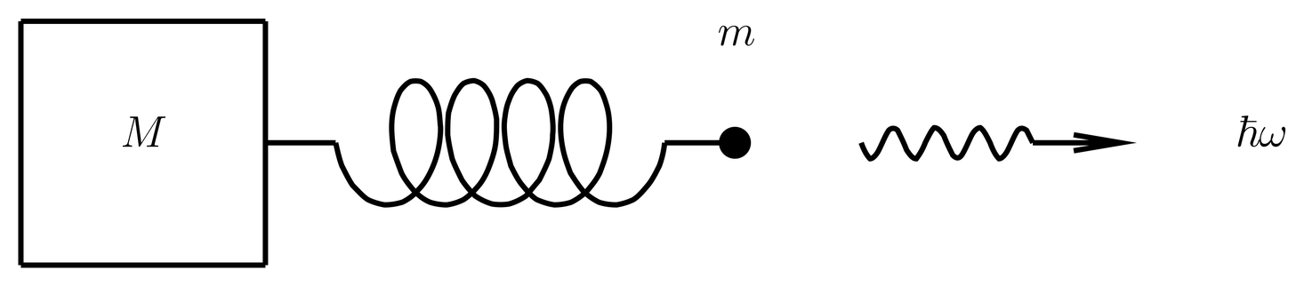
Figure 2:A one dimensional model of an iron atom coupled to a normal mode of the lattice. The mass of the iron atom is , the mass of the crystal is . The iron atom emits a photon of energy and suffers a recoil (an impulse) as a result.
To model this situation in the simplest possible way, let us imagine an iron atom connected to a spring, forming a one-dimensional harmonic oscillator, as illustrated in Figure 2. In the figure is the mass of the iron atom while is the mass of the crystal lattice to which it is coupled. When the atom emits a photon it suffers an an impulse, that is, a change in its momentum. The emission takes place over a short time compared to the frequency of the harmonic oscillator (a normal mode of the lattice), so the position of the iron atom does not change much during the emission process. Classically we can model the impulse by the map,
To model the effect of the recoil in quantum mechanics, we use the momentum displacement operator introduced in 08. Harmonic Oscillators and Coherent States{} [see (66)--(68)]. That is, if is the state of the oscillator before the photon is emitted, then the state after the emission is
The final state can be expanded in energy eigenstates,
so that the probability of finding the oscillator in state after the photon has been emitted is . In particular, if the initial state of the oscillator is an energy eigenstate, then the probability is the probability to make a transition as a result of the recoil. As we say, phonons are emitted. See Prob. Paragraph.
In fact, there is a certain probability that no phonons are emitted at all, that is and the oscillator remains in the initial state. Because of quantum mechanics, the recoil energy cannot take on any value, but rather is quantized, and the value zero is allowed. What makes the nucleus attractive for the M"ossbauer effect is that it has a reasonable probability for this recoilless emission.
Of course there is not only a recoil energy but also a recoil momentum. In the M"ossbauer effect, recoilless emission does not violate conservation of momentum because the entire crystal lattice, with an effectively infinite mass (as in the figure) takes up the recoil momentum.
The excited state has only a short lifetime but in practice a population of these excited states is maintained in the source as a part of the decay chain of , as shown in Figure 1. has a lifetime of 271 days, which is long enough to make it practical to use it as a source of in a real experiment. As shown in the figure, transforms into an excited state by electron capture, after which decays by the emission of a photon into , which is the source of the photons of interest in the M"ossbauer effect.
M"ossbauer was awarded the Nobel Prize in 1961 for his discovery of recoilless emission of gamma ray photons and some of its applications. A notable early application was the Pound-Rebka experiment, carried out in 1959, in which the M"ossbauer effect was used to make the first measurement of the gravitational red shift. This is the red shift photons experience when climbing in a gravitational field, in accordance with the 1911 prediction of Einstein. The gravitational red shift is one of the physical cornerstones of general relativity.
Energy levels in 
To return to the subject of Hamiltonians and their energy levels in isolated systems, let us draw attention to the three levels , and , in Figure 1. These are energy levels of the Hamiltonian for the nucleus, and, according to Theorem~Theorem, each must consist of one or more irreducible subspaces under rotations. In fact, each of them consists of precisely one such irreducible subspace, with a definite value, which is indicated in the figure ( for the ground state , and and for the two excited states and , respectively). Also indicated are the parities of these states (all three have odd parity). The parity of energy eigenstates of isolated systems is discussed in Parity and Energy Eigenstates in Isolated Systems.
A model for the Hamiltonian of the nucleus views it as a 57-particle system, that is, with 26 protons and 31 neutrons. The Hamiltonian is some function of the positions, momenta and spins of the particles,
where . In this model the total angular momentum of the system is the sum of the orbital and spin angular momenta of the nucleons,
and the “spins” of the various nuclear states shown in Figure 1 are actually the quantum numbers of (that is, we call the “spin” and use the notation etc.\null{} for it). For example, we say that the ground state has spin .
This model is more or less crude, due to the fact that protons and neutrons are composite particles, each made up of three quarks, which interact with the quark and gluon fields via the strong interactions. For our purposes the only thing that matters is that rotations act upon the state space of the system by means of unitary operators, and that these commute with the Hamiltonian. The model (47) at least gives us something concrete to think about.
Each nuclear energy eigenstate consists of a single irreducible subspace under rotations for the same reasons discussed in connection with central force motion in Energy Eigenstates in Isolated Systems. That is, extra degeneracy requires extra symmetry or else an unlikely accident, and neither of these is to be expected in nuclei. Therefore each energy level is characterized by a unique angular momentum value, as indicated in the figure.
We can summarize these accumulated facts by stating an addendum to Theorem~Theorem.
Addendum to Theorem 1.{\sl{} With a few exceptions, notably the electrostatic model of hydrogen, the bound state energy eigenspaces of isolated systems consist of a single invariant, irreducible subspace under rotations. Thus, the energy eigenvalues are characterized by an angular momentum quantum number, which is variously denoted , , , etc, depending on the system.}
We can now understand why the Hilbert space for spins in magnetic fields consists of a single irreducible subspace under rotations for a large class of particles, a question that was raised in 14. Spins in Magnetic Fields. For example, if we place the nucleus in a magnetic field that is strong by laboratory standards, say, 10T, then the energy splitting between the two magnetic substates will be of the order of 100~MHz in frequency units, or about , or roughly times smaller than the energy separation from the first excited state . Therefore it is an excellent approximation to ignore the state and all other excited states of the nucleus, and to treat the Hilbert space of the nucleus as if it were a single irreducible subspace with , that is, the ground eigenspace. In other words, in the case of nuclei, the -dimensional Hilbert space used in our study of spins in magnetic fields in 14. Spins in Magnetic Fields{} is actually a subspace of a larger Hilbert space. It is, in fact, an energy eigenspace of an isolated system. This in turn explains why the magnetic moment is proportional to the spin [see Prob. Paragraph(a)].
Problems
Problem 1.
Some questions on the M"ossbauer effect and the Pound-Rebka experiment.
The gravitational red shift is a prediction of general relativity, but the basic physics behind it can be understood in elementary terms. In the Pound-Rebka experiment, photons were launched upward from the ground, just outside a building at Harvard University. These photons were then received by a detector just outside the window of an upper floor of the building, approximately 20~meters above the ground.
Suppose at the very moment a photon is released at the ground, a physicist with a detector in hand jumps out of the upper storey window. As the photon is climbing upward in the earth’s gravitational field, suffering a red shift in the process, the physicist is falling, accelerating downward. At a certain point the detector captures the photon and the physicist measures its frequency. This frequency is blue shifted compared to what it would be if the physicist had just held the detector out the window, instead of jumping, because of the Doppler shift due to the downward motion of the detector.
It turns out that the gravitational red shift and the blue shift due to the falling detector (cum physicist) exactly cancel. Thus, the physicist finds a measured frequency of the photon exactly equal to the frequency it had when emitted at ground level. You can use this fact to calculate the gravitational red shift as seen by a detector that is just held out the window, not falling.
This situation is similar to that illustrated in the “shoot the monkey” demonstration used in elementary physics classes, except that instead of an arrow shot at the monkey particles of light are used. The basic physical reasoning used here is close to that employed by Einstein in his 1911 paper which first predicted the gravitational red shift.
(a) If an atom is free (not a part of a crystal lattice or otherwise bound to anything else), then it suffers some recoil on emitting a photon, which produces a shift in the frequency of the emitted photon. In the case of the 14.4~KeV photon emitted by the nucleus, calculate the fractional shift due to this recoil and compare to the natural line width.
(b) If the atom is free-floating in a gas at 300~K, calculate the average due to the Doppler shift due to the thermal motion of the atom.
(c) Calculate the for the gravitational red shift of the same photon climbing (as in the Pound-Rebka experiment) about 20 meters in the earth’s gravitational field, and compare to the due to the natural line width. You will see that the experiment was a delicate one that required careful measurement and attention to systematic errors.
Problem 2.
Consider a vector operator and a tensor operator .
(a) Show that if one component of } vanishes, then they all do.
(b) Is this true for a tensor operator ?