11. Rotations in 3-Dimensional Space
Introduction
The theory of rotations is of direct importance in all areas of atomic, molecular, nuclear and particle physics, and in large areas of condensed matter physics as well. The ideas developed in this and subsequent sets of notes on rotations in quantum mechanics will recur many times in this course, continuing through the second semester. The rotation group is the first nontrivial symmetry group we encounter in a study of quantum mechanics, and serves as a paradigm for other symmetry groups one may encounter later, such as the symmetry that acts on the color degrees of freedom in quantum chromodynamics. Furthermore, transformations that have the same mathematical form as rotations but which have nothing to do with rotations in the usual physical sense, such as isotopic spin transformations in nuclear physics, are also important. Rotations are also the spatial part of Lorentz transformations, and Lorentz invariance is one of the basic principles of modern physics. We will study Lorentz transformations in quantum mechanics in 48. Covariance of the Dirac Equation.
These notes will deal with rotations in ordinary 3-dimensional space, such as they would be used in classical physics. We will deal with quantum representations of rotations in 12. Rotations in Quantum Mechanics, and Rotations of Spin-1/2 Systems{} and \repsamos.
Inertial Frames
The concept of an inertial frame is the same in Newtonian (nonrelativistic) mechanics and in special relativity, both in classical mechanics and in quantum mechanics. It requires modification only in general relativity, that is, when gravitational fields are strong.
We define an inertial frame as a frame in which free particles (particles upon which no forces act) move in straight lines with constant velocity. An inertial frame has three mutually orthogonal axes, with respect to which coordinates of points can be measured. It assumed that the measurements of distance obey the rules of Euclidean geometry in three-dimensional space. This is a physical assumption that can be tested experimentally. In fact, the geometry of space is not exactly Euclidean, due to the effects of gravitational fields; but in weak fields the deviations are very small and we shall ignore them. It is another physical assumption that there exists a frame in which free particles move on straight lines with constant velocity, but given the existence of one such frame, a whole family of other inertial frames may be generated by applying translations, rotations and boosts. Rotating and/or accelerating frames are excluded by the requirement regarding the uniform, rectilinear motion of free particles.
Rotation Operators in Ordinary Space and Rotation Matrices
Let be the origin of an inertial frame, and let “points of space” be identified by their coordinates with respect to this frame. Points of space can also be identified by the vectors from to the points in question, as with vectors and in Figure 1.
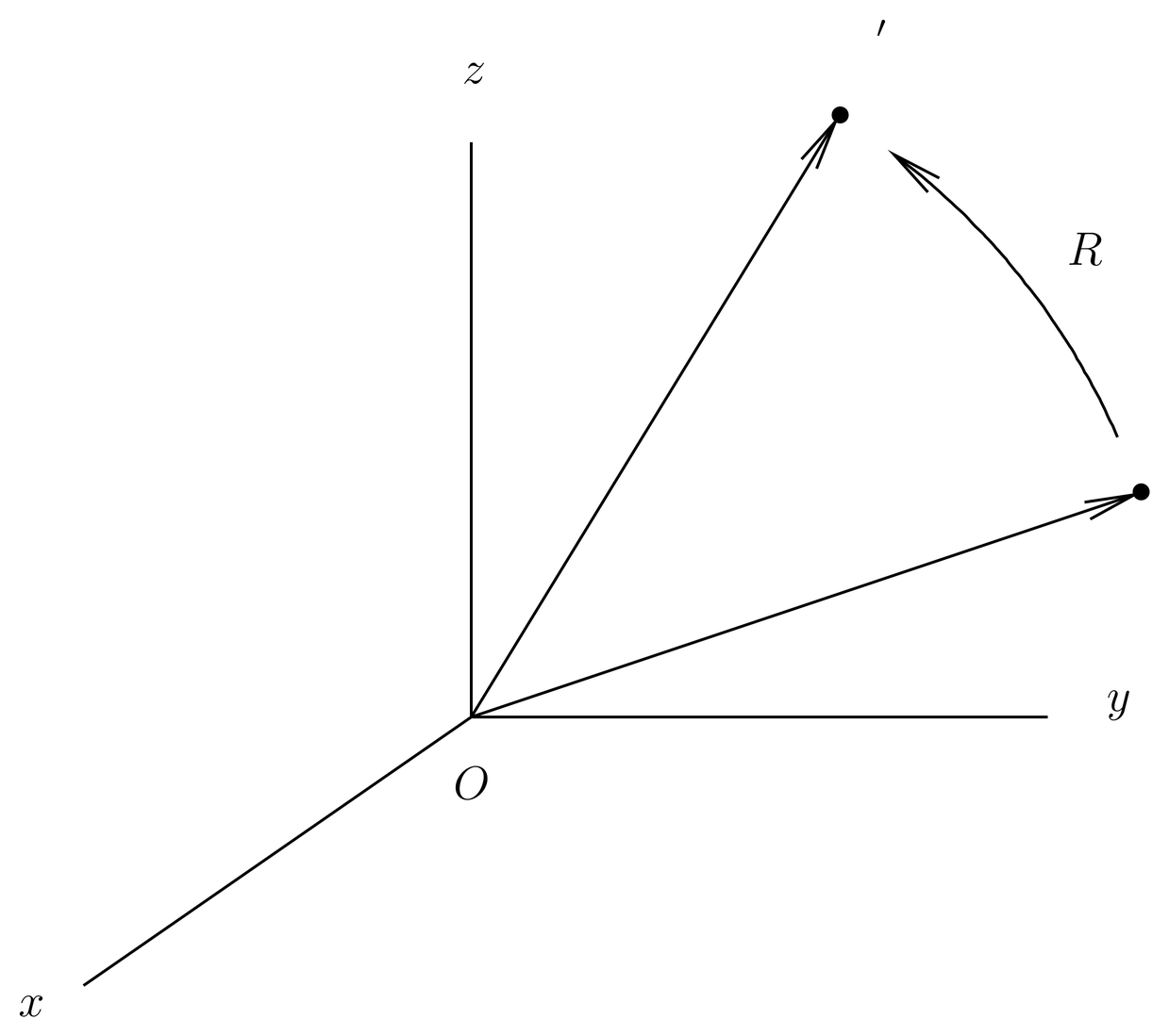
Figure 1:A rotation is defined as a map from space to itself that leaves one point invariant, while preserving all distances between points.
We define a rotation on ordinary space as a map that takes points of space into other points of space in such a way that is mapped into itself and all distances are preserved. In Figure 1, map takes point into point , so we can write
Since preserves distances it maps straight lines into straight lines and it satisfies
Also, since angles can be expressed in terms of distances, preserves angles, too. This means that maps parallelograms into congruent parallelograms, and since vector addition can be expressed in terms of parallelograms, it follows that
Combined with (2), this means that is a linear operator on ordinary space, regarded as a vector space. It also follows that is invertible, and thus exists. This is because a linear operator is invertible if the only vector it maps into the zero vector is itself, something that is satisfied in this case because is the only vector of zero length.
The product of two rotations is denoted , which means, apply first, then . Rotations do not commute in general, so that , in general. It follows from the definition that if , and are rotation operators, then so are and . Also, the identity operator is a rotation. These facts imply that the set of rotation operators forms a group.
We can describe rotations in coordinate language as follows. We denote the mutually orthogonal unit vectors along the axes of the inertial frame by or . We assume the frame is right-handed. Vectors such as or can be expressed in terms of their components with respect to these unit vectors,
Similarly, we define the rotation matrix associated with the operator by
where are the components of the matrix . (In these notes, we use sans serif fonts for matrices, but ordinary italic fonts for their components.) The definition (5) can be cast into a more familiar form if we use a round bracket notation for the dot product,
where and are arbitrary vectors. Then the definition (5) can be written,
This shows that are the matrix elements of with respect to the basis in the much same manner in which we define matrix elements of operators in quantum mechanics.
The definition (7) provides an association between geometrical rotation operators and matrices which depends on the choice of coordinate axes . If , and are rotation operators corresponding to , and , then corresponds to (multiplication in the same order) and corresponds to . As we say, the matrices form a representation of the geometrical rotation operators .
Assuming that and are related by the rotation as in Figure 1 or (1), we can express the components of in terms of the components of . We have
where we use the linearity of and the definition (7) of . We can write this in matrix-vector notation as
which looks just like (1) except that now , are seen, not as geometrical vectors as in Figure 1, but rather as triplets of numbers, that is, the coordinates of the old and new points with respect to the basis .
Active versus Passive Point of View
When dealing with rotations or any other symmetry group in physics, it is important to keep distinct the active and passive points of view. In this course we will adopt the active point of view unless otherwise noted. The active point of view is used by Messiah, Quantum Mechanics and Sakurai, Modern Quantum Mechanics, but many other books take the passive point of view, including some standard monographs on rotations, such as Edmonds, Angular Momentum in Quantum Mechanics. Books on classical mechanics usually take the passive point of view. The active point of view is usually preferable, because it is more amenable to an abstract or geometrical treatment, whereas the passive point of view is irrevocably chained to coordinate representations.
In the active point of view, we usually imagine one coordinate system, but think of operators that map old points into new points. Then an equation such as indicates that and are the coordinates of the old and new points with respect to the given coordinate system. This is the interpretation of (9) above. In the active point of view, we think of rotating our physical system but keeping the coordinate system fixed.
In the passive point of view, we do not rotate our system or the points in it, but we do rotate our coordinate axes. Thus, in the passive point of view, there is only one point, but two coordinate systems. To incorporate the passive point of view into the discussion above, we would introduce the rotated frame, defined by
and then consider the coordinates of a given vector with respect to the two coordinate systems and the relations between these components. In a book that adopts the passive point of view, an equation such as probably represents the coordinates and of a single point with respect to two (the old and new) coordinate systems. With this interpretation, the matrix has a different meaning than the matrix used in the active point of view [such as that in (9) and elsewhere in these notes], being in fact the inverse of the latter. Therefore caution must be exercised in comparing different references. In this course we will make little use of the passive point of view.
Properties of Rotation Matrices; the Group 
Since the rotation preserves lengths, we have
when , are related by (9). Since this is true for arbitrary , we have
This is the definition of an orthogonal matrix. The set of all real orthogonal matrices is denoted in standard notation, so our rotation matrices belong to this set. In fact, since every orthogonal matrix in corresponds to a rotation operator by our definition, the space of rotations is precisely the set . The set forms a group under matrix multiplication that is isomorphic to the group of geometrical rotation operators introduced above.
(12) implies
so that it is easy to invert an orthogonal matrix. This in turn implies
[in the reverse order from (12)]. Taken together, (12) and (14) show that the rows of an orthogonal matrix constitute a set of orthonormal vectors, as do the columns.
Proper and Improper Rotations; the Group 
Taking determinants, (12) also implies , or
Orthogonal matrices for which are said to be proper rotations, while those with are said to be improper. Proper rotations have the property that they preserve the sense (right-handed or left-handed) of frames under the transformation (10), while improper rotations reverse this sense.
The set of proper rotations by itself forms a group, that is, the property is preserved under matrix multiplication and inversion. This group is a subgroup of , denoted , where the stands for “special,” meaning in this case . The set of improper rotations does not form a group, since it does not contain the identity element. An improper rotation of some importance is
which inverts vectors through the origin.
For the duration of these notes we will restrict consideration to proper rotations whose matrices belong to the group , but we will return to improper rotations in 21. Parity.
Rotations About a Fixed Axis; the Axis-Angle Parameterization
Let us consider now a proper rotation which rotates points of space about a fixed axis, say, , by an angle , in which the sense is determined by the right-hand rule. See Figure 2. We will denote this rotation by and the matrix by . It is geometrically obvious that rotations about a fixed axis commute,
and the angles add under matrix multiplication as indicated. The rotations about the three coordinate axes are of special interest; these are
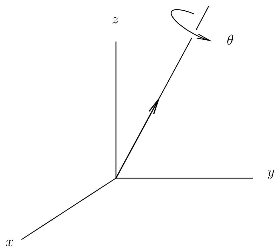
Figure 2:A proper rotation is specified by a unit vector that defines an axis, and a rotation of angle about that axis. The rotation follows the right-hand rule.
One can show that any proper rotation can be represented as , for some axis and some angle . Thus, there is no loss of generality in writing a proper rotation in this form. We will call this the axis-angle parameterization of the rotations. This theorem is not totally obvious, but the proof is not difficult (see Prob.~\prbrclassrot-4). It is based on the observation that every proper rotation must have an eigenvector with eigenvalue +1. This eigenvector or any multiple of it is invariant under the rotation and defines its axis.
Infinitesimal Rotations
A rotation that is close to the identity is called near-identity or infinitesimal. It has the form
where is a small scale factor whose purpose is to make the correction term small, and where is a matrix. By substituting (19) into the orthogonality condition (12), we find
that is, the matrix is antisymmetric.
A convenient parameterization of the antisymmetric matrices is given by
where is a “vector” of matrices, defined by
Equations~(22) can be summarized by writing
We will also write the sum in (21) as , that is, as a dot product of vectors, but we must remember that is a triplet of ordinary numbers, while is a triplet of matrices. The notation is similar to that which we use with the Pauli matrices, a “vector” of matrices. See Prob. Paragraph.
(21) associates an antisymmetric matrix with a corresponding 3-vector . In the following we will find it convenient to switch back and forth between these representations.
A useful property of the matrices is the following. Let be an antisymmetric matrix, associated with a vector according to (21), and let be another vector. Then
Now taking the -th component of the right-hand side and using (23), we find
where we use the summation convention. In other words,
This gives us an alternative way of writing the cross product (as a matrix multiplication) that is often useful.
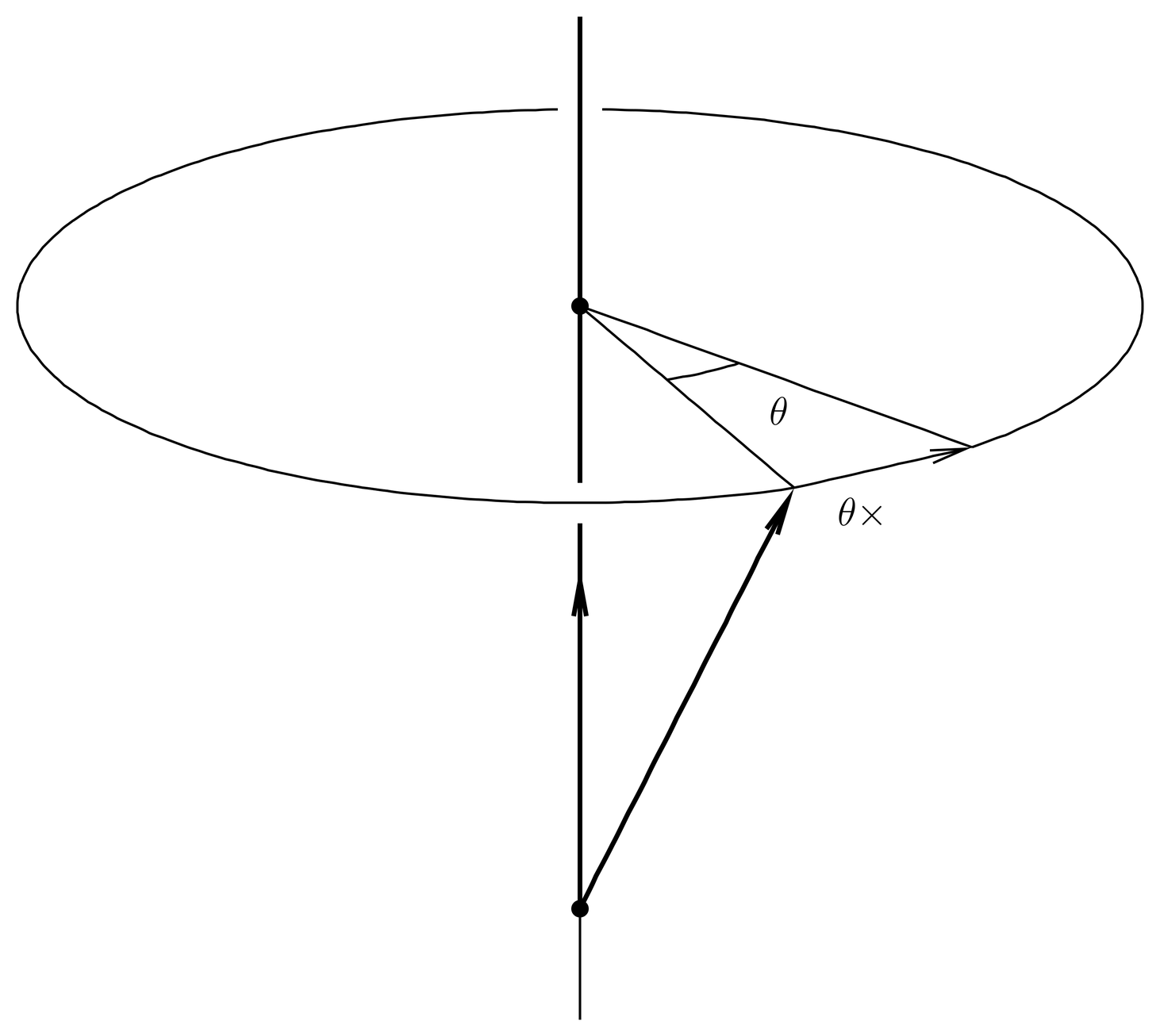
Figure 3:The effect of a near-identity rotation of small angle about axis on a vector is to move it by the amount .
Since every proper rotation has an axis and an angle, we can ask, what are the axis and angle of the near-identity rotation (19)? To find out, we write
which implies
where is an arbitrary vector. But another way of writing this equation appears when we examine Figure 3, which shows the action of a rotation about axis by small angle on the same vector . The result is
Comparing this with (28), we see that the axis and angle of an infinitesimal rotation is given in terms of the correction matrix in (19) by
or,
The result is a useful expression for an infinitesimal rotation in axis-angle form,
We tabulate here some useful properties of the matrices [see also (23) and (26)]. First, the product of two matrices can be written,
as follows from (23)and (53). From this there follows the commutation relation,
or
The commutation relations (34) obviously resemble the commutation relations for angular momentum operators in quantum mechanics, but without the . As we shall see, the quantum angular momentum commutation relations are a reflection of these commutation relations of the matrices at the classical level. Ultimately, these commutation relations represent the geometry of Euclidean space.
Exponential Form of Finite Rotations
We will now establish a connection between infinitesimal rotations and the finite rotations which take place about a fixed axis. The argument is similar to the one given previously in connection with translation operators [see (38) and (39)].
Our strategy is to set up a differential equation for and to solve it. By the definition of the derivative, we have
But according to (17), the first factor in the numerator can be written
so the derivative becomes
In the limit, becomes a small angle, so we can use (32) to evaluate the limit, obtaining,
Solving this differential equation subject to the initial conditions , we obtain
This exponential can be expanded out in a power series that carries (32) to higher order terms,
This series converges for all values of and .
The same result can be obtained in another way that is more pictorial. It is based on the idea that a rotation about a finite angle can be built up out of a sequence of small angle rotations. For example, a rotation of one radian is the product of a million rotations of 10-6 radians.
Let us take some angle and break it up into a product of rotations of angle , where is very large:
We can make as small as we like by making large. Therefore we should be able to replace the small angle rotation in (42) by the small angle formula (32), so that
This is a limit of matrices that is similar to the limit of numbers shown in (46). It turns out that the matrix limit works in the same way, giving (40).
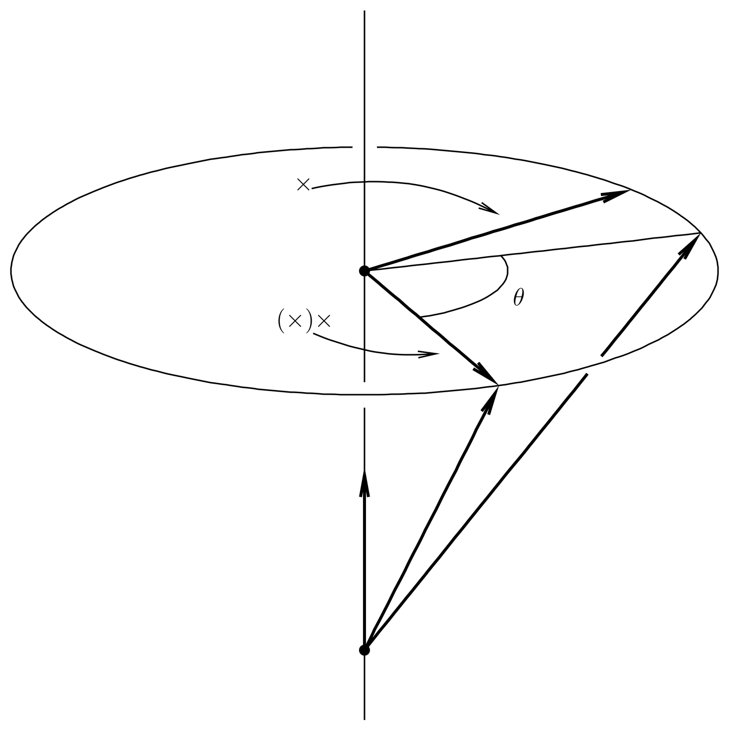
Figure 4:The result of applying a finite rotation to a vector can be expressed as a linear combination of the vectors , , and , the latter two of which are orthogonal.
Explicit Form for Action of Rotation on a Vector
Finite rotations about a fixed axis can be expressed in another way. By using the properties of the matrices listed above, one can express higher powers of the matrix in terms of lower powers, and reexpress the the exponential series (40), acting on an arbitrary vector , in the following form:
The geometrical meaning of this formula is easy to see; the rotation about leaves the component of parallel to invariant, and rotates the component perpendicular to by an angle in the perpendicular plane. This is illustrated in Figure 4.
Adjoint Formulas
Let and be arbitrary vectors, and consider how the cross product transforms under proper rotations. For a proper rotation , the rule is
or, as we say in words, the cross product transforms as a vector under proper rotations. The proof of (45) will be left as an exercise (see Prob.~\prbrclassrot-2), but if you do it, you will find it is equivalent to . In fact, if is improper, there is a minus sign on the right hand side, an indication that the cross product of two true vectors is not a true vector, but rather a pseudovector. More on this in 21. Parity, when we return to the improper rotations and discuss parity in quantum mechanics.
Now let us use the notation (26) to express the cross products in (45) in terms of matrix multiplications. This gives
or, since is arbitrary,
We now multiply through on the right by , obtaining,
This formula is of such frequent occurrence in applications that we will give it a name. We call it the adjoint formula, because of its relation to the adjoint representation of the group .
Let us now replace by to avoid confusion with other rotation matrices to appear momentarily, and let us replace by for the axis and angle of a rotation. Then exponentiating both sides of the adjoint formula (48), we obtain,
where we have used the rule,
valid for matrices or operators and when exists. This rule can be verified by expanding the exponential series. The result (49) can be written,
We will call this the exponentiated version of the adjoint formula.
The exponentiated version of the adjoint formula (51) says that the axis of a rotation transforms as a vector under proper rotations, while the angle of rotation does not change. As with the original version of the adjoint formula (48), this only holds for proper rotations. (51) might be easier to understand in a passive interpretation, in which is used to transform the components of to a new basis. The new matrix is obtained simply by transforming the axis to the new basis, while keeping the angle fixed.
Group Manifolds for and 
We turn now to the question of parameterizing the rotation matrices or rotation operators. Since an arbitrary, real matrix contains 9 real parameters, and since the orthogonality condition constitutes 6 constraints, it follows that it will take 3 parameters to specify a rotation. This is clear already from the axis-angle parameterization of the rotations, since an axis is equivalent to two parameters (say, the spherical angles specifying the direction of ), and the angle of rotation is a third parameter.
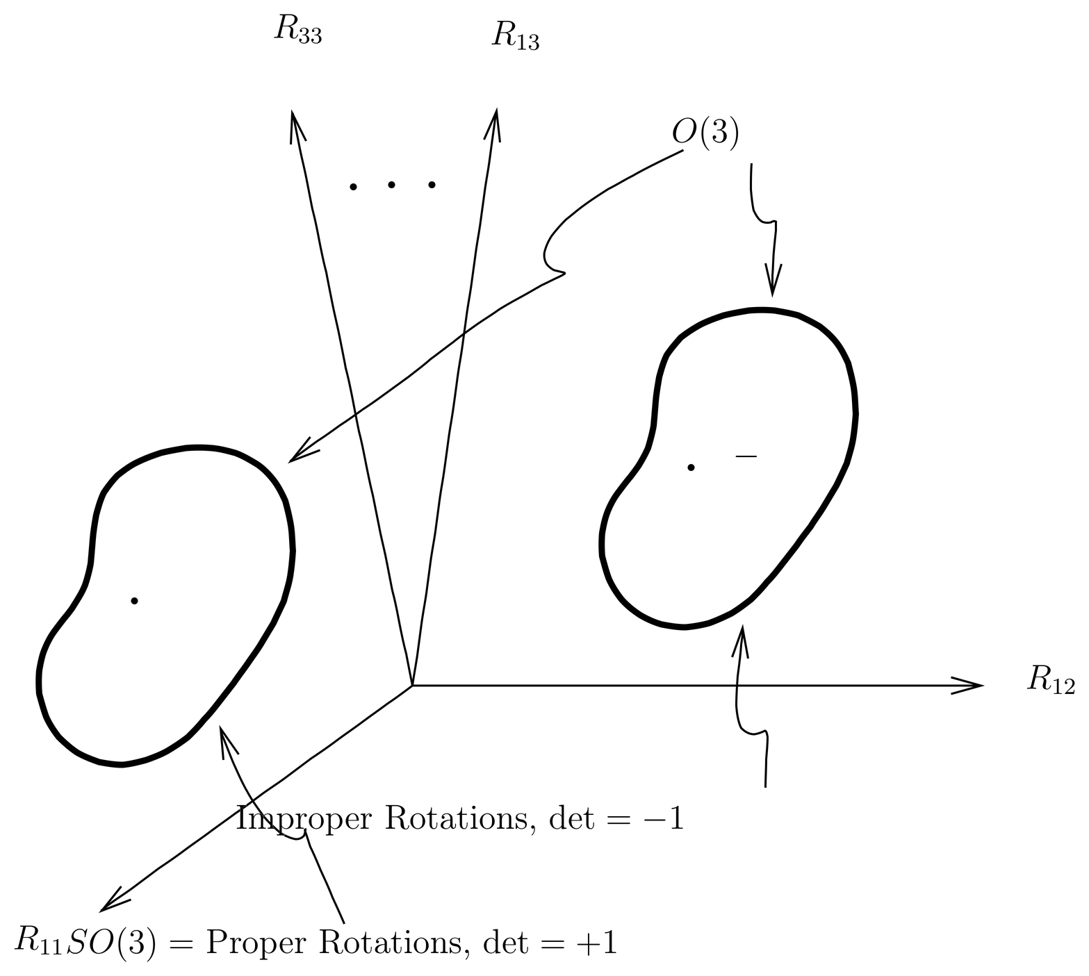
Figure 5:The rotation group can be thought of as a 3-dimensional surface imbedded in the 9-dimensional space of all matrices. It consists of two disconnected pieces, one of which contains the proper rotations and constitutes the group , and the other of which contains the improper rotations. The proper rotations include the identity matrix , and the improper rotations include the parity matrix .
It is often useful to think of the rotations and their parameters in geometrical terms. We imagine setting up the 9-dimensional space of all real matrices, in which the coordinates are the components of the matrix, . It is difficult to visualize a 9-dimensional space, but we can use our imagination as in Figure 5. The 6 constraints implicit in imply that the orthogonal matrices lie on a 3-dimensional surface imbedded in this space. This surface is difficult to draw realistically, so it is simply indicated as a nondescript blob in the figure. More exactly, this surface consists of two disconnected pieces, containing the proper and improper matrices. This surface (both pieces) is the group manifold for the group , while the piece consisting of the proper rotations alone is the group manifold for . The identity matrix occupies a single point in the group manifold , while the improper matrix lies in the other piece of the group manifold . Any choice of three parameters for the proper rotations can be viewed as a coordinate system on the group manifold .
The group manifolds and are bounded, that is, they do not run off to infinity. The topological designation for this is that the manifolds are compact. This follows from the fact that every row and column of an orthogonal matrix is a unit vector, so all components lie in the range .
The group manifold is the configuration space for a rigid body. This is because the orientation of a rigid body is specified relative to a standard or reference orientation by a rotation matrix that maps the reference orientation into the actual one. In classical rigid body motion, the orientation is a function of time, so the classical trajectory can be seen as a curve on the group manifold . In quantum mechanics, a rigid body is described by a wave function defined on the group manifold . Many simple molecules behave approximately as a rigid body in their orientational degrees of freedom.
Euler Angles
In addition to the axis-angle parameterization of the rotations, another important parameterization is the Euler angles. To construct the Euler angles, let us return to the frame introduced at the beginning of these notes, and recall the rotated frame defined in (10). We will take it as geometrically obvious that the rotation operator or the corresponding rotation matrix is uniquely specified by the orientation of the rotated frame. Therefore to obtain parameters of the rotation, we can specify the orientation of the rotated frame, that is, the orientation of all three rotated axes.
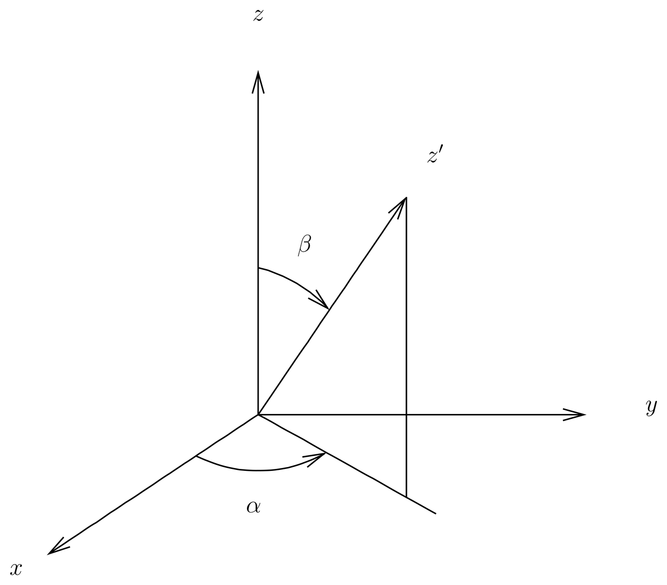
Figure 6:The Euler angles and are the spherical angles of the rotated -axis as seen in the unrotated frame.
We begin by specifying the orientation of the rotated -axis. This axis points in some direction, which we can indicate by its spherical angles, say, , with respect to the unrotated frame. This is illustrated in Figure 6. We have in mind here some rotation , which corresponds to definite orientations of the three primed axes. The rotation maps the old (unprimed axes) into the new (primed) ones, and in particular, it satisfies . Another rotation matrix that also maps the old -axis into the new -axis is , defined by
By examining Figure 6, it is easy to see that satisfies
since the first rotation by angle about the -axis swings the -axis down in the - plane, and then the second rotation by angle about the -axis rotates the vector in a cone, bringing it into the final position for the -axis. Rotation is not in general equal to , for is only designed to orient the -axis correctly, while puts all three primed axes into their correct final positions. But can get the - and -axes wrong only by some rotation in the - plane; therefore if we follow the and rotations by a third rotation by some new angle, say, , about the -axis, then we can guarantee that all three axes achieve their desired orientations. That is, we can write an arbitrary rotation in the form,
for some angles .
But it is not convenient to express a rotation in terms of elementary rotations about a mixture of old and new axes, as in (54); it is more convenient to express it purely in terms of rotations about the old axes. To do this, we write
using the exponentiated version of the adjoint formula (51). Therefore
This gives us the Euler angle parameterization of proper rotations,
It is a factorization of an aribtrary, proper rotation into a product of rotations about the coordinate axes, taken in the order .
(57) constitutes the -convention for the Euler angles, which is particularly appropriate for quantum mechanical applications. Other conventions are possible, and the -convention is common in books on classical mechanics, while the -convention is used in aeronautical engineering (the three rotations are called pitch, yaw and roll, familiar to airplane pilots). Also, you should note that most books on classical mechanics and some books on quantum mechanics adopt the passive point of view, which usually means that the rotation matrices in those books stand for the transposes of the rotation matrices in these notes.
The geometrical meanings of the Euler angles and is particularly simple, since these are just the spherical angles of the -axis as seen in the unprimed frame. The geometrical meaning of is more difficult to see; it is in fact the angle between the -axis and the unit vector lying in the line of nodes. The line of nodes is the line of interbetween the - plane and the - plane. This line is perpendicular to both the - and -axis, and we take to lie in the direction .
The allowed ranges on the Euler angles are the following:
The ranges on and follow from the fact that they are spherical angles, while the range on follows from the fact that the -rotation is used to bring the - and -axes into proper alignment in their plane. If the Euler angles lie within the interior of the ranges indicated, then the representation of the rotations is unique; but if one or more of the Euler angles takes on their limiting values, then the representation may not be unique. For example, if , then the rotation is purely about the -axis, and depends only on the sum of the angles, . In other words, apart from exceptional points at the ends of the ranges, the Euler angles form a 1-to-1 coordinate system on the group manifold .
The Noncommutativity of Rotations
As pointed out earlier, rotations do not commute, so , in general. An exception, also noted above, is the case that and are about the same axis, but when rotations are taken about different axes they generally do not commute. Because of this, the rotation group is said to be non-Abelian. This means that the rotation group is noncommutative.
Let us write and for two rotations in axis-angle form. If the axes and are not identical, then it is not entirely simple to find the axis and angle of the product, that is, and in
A formula for and in terms of the axes and angles of and exists, but it is not trivial. If we write
for the three antisymmetric matrices in the exponential expressions for the three rotations in (61), then that equation can be written as
and the problem is to find in terms of and . We see once again the problem of combining exponentials of noncommuting objects (matrices or operators), one that has appeared more than once previously in the course. We comment further on this problem below.
The situation is worse in the Euler angle parameterization; it is quite a messy task to find in terms of and in the product,
The difficulties of these calculations are due to the noncommutativity of the rotation matrices.
A measure of the commutativity of two rotations , is the matrix
which itself is a rotation, and which becomes the identity matrix if and should commute. The matrix is more interesting than the ordinary commutator, , which is not a rotation. You can think of as taking a step in the 1-direction, then a step in the 2-direction, then a backwards step in the 1-direction, and finally a backwards step in the 2-direction, all in the space of rotations, and asking if we return to the identity. The answer is that in general we do not, although if the steps are small then we trace out a path that looks like a small parallelogram that usually does not quite close.
Let us examine when the angles and are small. Let us write for the antisymmetric matrices in the exponents of the exponential form for the rotations, as in (62), and let us expand the exponentials in power series. Then we have
The first order term vanishes, and at second order we find the commutator of the matrices, as indicated. Writing these in terms of axes and angles as in (62), the matrix becomes
where we have used the commutation relations (35). We see that if and are near-identity rotations, then so is , which is about the axis .
Matrix is a near-identity rotation, so we can write it in axis-angle form, say, with axis and angle ,
Comparing this with (67), we have
This result will be of use in 12. Rotations in Quantum Mechanics, and Rotations of Spin-1/2 Systems.
The Baker-Campbell-Hausdorff Theorem
It is no surprise to see the commutator of near identity rotations expressed in terms of the commutators of the matrices, since the latter are the correction terms for near identity rotations. (67) just gives the details. But there is an important point to be made about the commutation relations of near identity transformations, related to the Baker-Campbell-Hausdorff theorem, which we now discuss.
The theorem concerns products of exponentials of operators or matrices that need not commute, as in (63). We rewrite that equation in a different notation,
where and are given and it is desired to find . First, if and commute, then the product of exponentials follows the rules for ordinary numbers, and . Next, if and do not commute but they do commute with their commutator, then the conditions of Glauber’s theorem hold (see Heisenberg Operators and Glauber’s Theorem) and we have
If and do not commute with their commutator, then no simple answer can be given, but we can expand in a power series in and . Carried through third order, this gives
The Baker-Campbell-Hausdorff theorem concerns this series, and asserts that the general term of this Taylor series can be written in terms of commutators and iterated commutators of and . This fact can be seen through third order in (72). Thus, if we know how to compute commutators, we can in principle compute all the terms of this Taylor series and obtain the multiplication rule for products of exponentials.
For example, in the case of the rotations, knowledge of the commutation relations (34) or (35) allows us to compute all the terms of the Taylor series (72) and thus obtain the multiplication law for finite rotations in terms of axis-angle parameters, at least in principle. We do not intend to do this in practice, and in fact we shall use the Baker-Campbell-Hausdorff theorem only for its suggestive and intuitive value. But the point is that all the complexity of the noncommutative multiplication law for finite rotations is implicitly contained in the commutation relations of infinitesimal rotations, that is, of the matrices. This explains the emphasis placed on commutation relations in these notes and in physics in general.
Problems
Problem 1.
Prove the commutation relations (\eqr\cn.34), using Eq.~(\eqr\cn.23) and the properties of the Levi-Civita symbol . See Sec.~\secr\tensor.16.
Problem 2.
Some useful identities.
(a) Show that if }, then
Also show that
These formulas hold for all vectors and .
(b) Show that if , then
Hint: Use the fact that if is any matrix, then
This is essentially the definition of the determinant. This proves (45), and hence the adjoint formulas (48) and (51). Note that when (76) is combined with (73), we obtain
valid for all and all vectors , and .
Problem 3.
The geometrical meaning of Eq.~(\eqr\cn.44) is illustrated in Fig.~\figr\cn.4. The rotation leaves the component of along the axis invariant, while rotating the orthogonal component in the plane perpendicular to .
By expressing powers of the matrices in terms of lower powers, sum the exponential series (40) and obtain another proof of (44).
Problem 4.
The axis of a proper rotation is invariant under the action of , that is, . Therefore is a real, normalized eigenvector of with eigenvalue +1.
Prove that every proper rotation has an axis. Show that the axis is unique (apart from the change in sign, ) as long as the angle of rotation is nonzero. This proof is the essential step in showing that every rotation can be expressed in axis-angle form. Do proper rotations in 4 dimensions have an axis?
Problem 5.
It is claimed that every proper rotation can be written in Euler angle form. Find the Euler angles for the rotation .