Appendix B. Classical Mechanics
Introduction
In this Appendix we summarize some aspects of classical mechanics that will be relevant for our course in quantum mechanics. We concentrate on the Lagrangian and Hamiltonian formulation of classical mechanics.
Lagrangians, Dissipation, and Entropy
In this Appendix we consider exclusively classical systems that can be described by a Lagrangian. This means that we neglect friction and other dissipative processes that cause an increase in entropy. Dissipation is always present in macroscopic systems, so its neglect is an approximation that is more or less good depending on circumstances.
The concept of entropy applies when making a statistical description of a system, which is often necessary when the number of degrees of freedom is large. Entropy provides a measure of our ignorance of the state of the system, that is, of the values of the dynamical variables that describe the system.
In some macroscopic systems it is a good approximation to concentrate on just a few degrees of freedom that we are interested in, and to neglect interactions with a large number of other degrees of freedom that we do not care about. For example, in the motion of a planet around the sun we may wish to describe the position of the center of mass of the planet in detail while ignoring its rotations as well as the internal stresses inside the solid body of the planet, the bulk motions of fluids in its oceans and atmospheres, etc. The latter are macroscopic degrees of freedom that are in turn coupled to microscopic ones, the motions of the individual atoms and molecules that make up the planet. There is a chain of couplings leading from macroscopic degrees of freedom down to microscopic ones, and a corresponding transport of energy from large motions down to small ones, ultimately resulting in the production of heat.
If the couplings at any stage are small it may be possible to neglect them, to obtain a closed system with few degrees of freedom. This would certainly simplify the problem and may be valid over short periods of time. But over longer periods dissipation will be important and cannot be ignored. For example, ancient dissipative processes inside the body of the moon have caused it to settle into a state in which its rotation is synchronized with its revolution, so that we see only one face of it from the earth. And the tides in the earth’s oceans lead to dissipation of energy in the earth-moon system, causing the day to become longer while the moon recedes from the earth. (The energy required to move the moon away from the earth comes from the kinetic energy of the earth’s rotation. Conservation of angular momentum requires that the moon recede in this process.) The earth-moon system is heading toward a state in which the length of the day and the length of the month are equal.
Similar concepts apply to a block sliding across a table. Friction causes the kinetic energy of the block to be converted into heat in the block and the table, that is, into the energy of motion of the individual atoms and molecules of the block and table. If friction is small, we may neglect it and treat the block as if its center of mass or center of mass and orientation were isolated degrees of freedom, not interacting with any other.
If we do wish to take friction into account in the motion of a block sliding across a table, we may do so while limiting ourselves to a small number of degrees of freedom by using a phenomenological force law, for example, one that says that the frictional force is , where and are constants and where is the velocity of the block. Such force laws may have some theoretical justification or may be just fits to experimental data. They amount to taking into account the large number of internal degrees of freedom of the block and table in an average way. It is straightforward to write down Newton’s laws , including such frictional forces, to obtain differential equations for the motion of the few degrees of freedom we are interested in. Such frictional force laws, however, preclude a Lagrangian formulation of the system.
In this course we will be especially interested in microscopic systems with a small number of degrees of freedom, whose dynamics we will follow in detail, that is, without using statistics. Such systems are sometimes isolated from their environment, so it is not hard to write down equations of motion for their internal dynamics. An example is an atom or molecule in a low-density gas between collisions. Since such systems only have a small number of degrees of freedom, there is no question of any coupling to a large number of “internal” degrees of freedom, as in the case of the block. If the system is not isolated, however, then it does interact with “external” degrees of freedom, that is with external fields (gravitational, electromagnetic, etc).
In such cases we will assume that the external fields are simply given as a function of space and time. In reality, external fields are never known precisely, for example, a magnetic field produced by a current in some coils has fluctuations due to the finite temperature of the source of the current and of the coils themselves. In this course, we shall ignore such effects.
In summary, we shall ignore dissipative effects in this course, so that a Lagrangian description is possible. Systems that can be described by a Lagrangian include classical systems of point particles, fluids, elastic media and fields, both in nonrelativistic and relativistic mechanics. We begin with the nonrelativistic mechanics of systems of point particles.
Constrained Systems, Configuration Space, and Generalized Coordinates
In a system with particles, the positions of all the particles relative to an inertial frame are specified by coordinates, , or for short. Sometimes the positions of the particles are subject to constraints, for example, if a particle is sliding on the surface of a sphere of radius , its position coordinates are subject to the constraint . Or if the particles make up a rigid body, then the distances between any two particles is constant,
for all . Constraints appear both in classical mechanics and in quantum mechanics, for example, many small molecules are approximately rigid bodies.
Constrained systems are idealizations of systems with a larger number of degrees of freedom, in which strong confining forces cause the particles to move on or near the constraint surface. For example, a particle sliding on the surface of a sphere of radius can be thought of as a particle that feels a strong restoring force if it moves away from the surface in three-dimensional space.
Interesting issues arise when exploring such models in detail to see how the simple picture of constrained dynamics emerges from a more realistic model with strong constraining forces. For example, one finds that if the initial position is on the constraint surface and the initial velocity is tangent to it, then the position remains on the constraint surface at later times, to a good approximation when the constraining forces are strong. When the initial position is not on the constraint surface or the initial velocity is not tangent to it, then there are high-frequency oscillations about the constraint surface and the dynamics along the constraint surface are modified. This is an interesting chapter in adiabatic theory that we shall not pursue here, although we will touch on adiabatic problems in the course (see 39. Adiabatic Invariance, the Geometric Phase, and the Born-Oppenheimer Approximation).
In the case of constraints, the positions of the particles are described by some number of coordinates, call them . For example, in the case of the particle sliding on the sphere we have and we can take , the usual spherical coordinates on the sphere. In the case of the rigid body with one point fixed we have and we can take , the Euler angles of a rotation that maps a standard orientation of the rigid body into the actual orientation. See Euler Angles for the definition of Euler angles. In the case of a rigid body whose center of mass is free to move (for example, in a model of a planet), we have and coordinates , where are the coordinates of the center of mass. In general, the positions of the particles are functions of the ’s,
If the constraints are time-dependent, then these functions depend on time as indicated. For example, in the case of a particle sliding on a sphere of radius we have
If there are no constraints, then we have and we can take , that is, we can let the ’s be the rectangular coordinates of the particles. We may choose not to do this, however, for example, in the case of a single particle moving in three-dimensional space we may wish to use spherical coordinates and choose .
In general (with or without constraints), the ’s are coordinates on configuration space, an abstract space in which a single point represents the positions of all the particles of the system. The number of the ’s, which is the dimension of configuration space, is called the number of degrees of freedom. In the case of a single particle moving in three-dimensional space, configuration space is the same as physical space, but in general configuration space is best regarded as an abstract space. Here are two examples of configuration spaces. The configuration space of a system of unconstrained particles is , while the configuration space of a rigid body with one point fixed is the rotation group manifold (see 11. Rotations in 3-Dimensional Space).
The coordinates , , are called generalized coordinates. The word “generalized” simply means that the coordinates need not be rectangular coordinates. For constrained systems such as the particle sliding on a sphere, rectangular coordinates are not an option and all coordinates are “generalized.”
Variational Principles in Optics
It has been known for a long time that certain problems in optics can be expressed in terms of a variational principle. Consider, for example, the laws of reflection from a mirror, which state that the angle of incidence is equal to the angle of reflection. See Figure 1, in which a light ray leaves point , reflects off the mirror at point , and then reaches point . The actual path taken by the light ray on going from to , path in the figure, is the one that minimizes the total distance of travel. For example, the dotted path is longer. But the shortest path is also the one for which the angle of incidence is equal to the angle of reflection ( in the figure).
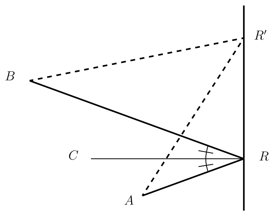
Figure 1:The actual path taken by a light ray when reflecting from a mirror, , is the one that minimizes the total distance traveled.
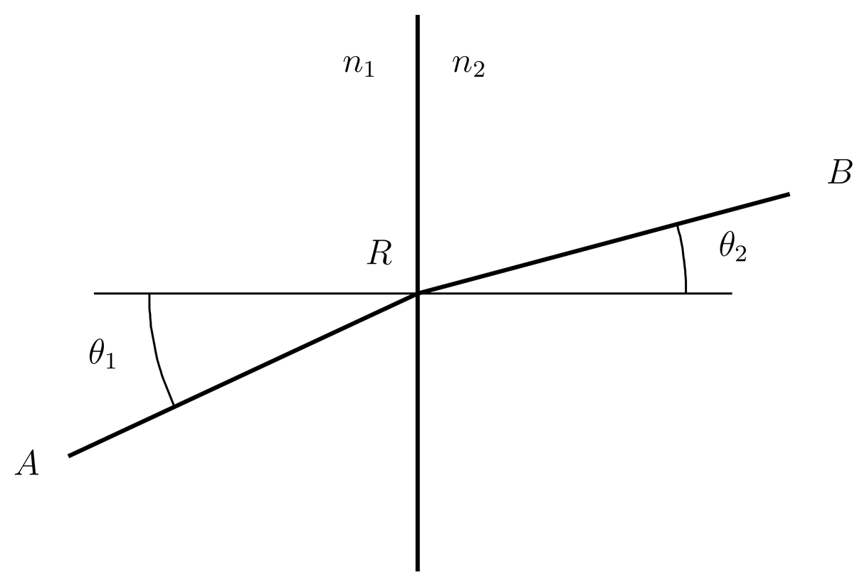
Figure 2:The path taken by the light ray on passing from one medium with index of refraction to another with index of refraction minimizes the quantity .
Similarly, the laws of refraction (Snell’s law) can be cast into a variational form. See Figure 2, in which there are two media with indices of refraction and . In this case it is not the total distance that is minimized, but the distance multiplied by the index of refraction. That is, the actual path, in the figure, is the one that minimizes , where is the distance from to a point on the interface, and is the distance from that point to . It can be shown that this path is one that satisfies Snell’s law,
In both these cases there is a space of paths over which the minimization takes place. In the case of the mirror, the space of paths consists of all paths that connect to a point on the mirror by a straight line, and then connect that point to by another straight line. This is a 2-parameter space of paths, because the mirror is a 2-dimensional surface (the parameters are the coordinates on the surface of the mirror). But the space of paths can be enlarged to include arbitrary, curved paths that join to , staying on one side of the mirror and touching it once, as in Figure 3. The actual path still has the minimum length, because all curved paths between any two points are longer than the straight path between those points. The enlarged path space is infinite-dimensional. Similarly, in the refraction problem illustrated in Figure 2, the space of paths can be enlarged to include curved paths that cross the interface only once.
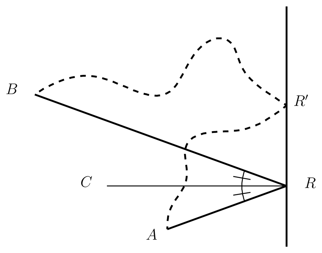
Figure 3:The space of paths reflecting from the mirror can be enlarged to include curved paths, and the actual path still minimizes the distance.
A more general situation is one in which the index of refraction is a function of position, , for example, when a light ray passes through the earth’s atmosphere. In this case it can be shown that the actual path taken by the light ray is one that minimizes the integral,
where the path is parameterized by the arc length . This integral is the generalization of the sum used in the refraction example above. In this case the space of paths consists of all paths that join given points and . The actual path satisfies the differential equation,
which is the Euler-Lagrange equation (see \secrclassmech-7) for the variational problem defined by (5).
The quantity in (5) is a functional of the path, and it is not obvious why it should be minimized along the actual path. A justification can be given by applying the short wavelength or WKB approximation to Maxwell’s equations in a slowly varying medium, but that does not make the form of the functional intuitive, nor does it explain why nonphysical paths should enter into a physical formulation of the problem. That is, the question arises, if the actual path followed by the light ray minimizes a certain quantity, does nature somehow know about the nonphysical paths in order to reject them? There is no answer purely within classical theory. As discussed in 09. The Propagator and the Path Integral, however, a more satisfactory justification comes from quantum mechanics. Suffice it to say here that in books the functional is often multiplied by , whereupon it becomes the time required for a particle to move along the light ray at the phase velocity . That is, it becomes a time functional,
Thus, one can say that the actual path minimizes the time, defined in this way. Why the phase velocity should appear here rather than the group velocity (which is the actual velocity at which signals propagate) is however a mystery.
Actually, the physical path does not always minimize the time. More generally it is a critical or stationary point of the time functional, that is, the physical path satisfies
The first functional derivative of the time functional with respect to the path vanishes on the physical path.
Critical Points
In elementary calculus, if we wish to find the extrema of a function of several variables, we first find the roots of
that is, we look for the places where the gradient of vanishes. These roots are called the critical points of the function . We can describe a critical point in words by saying small variations about the critical point give rise to only second order variations in the value of the function (the first order variations vanish).
Critical points are candidates for extrema. To find out if one is an extremum and of what type, we may examine the second derivative matrix evaluated at the critical point,
This matrix is real and symmetric, so its eigenvalues are real. If the eigenvalues are all positive, then the critical point is a minimum, that is, small variations about the critical point can only increase the value of the function. In general the minimum is only local, that is, there may be other minima with smaller values of at some distance away. If all the eigenvalues of the matrix (10) are negative, then the critical point is a (generally local) maximum. If some are negative and some are positive, then the critical point is a saddle. And if some eigenvalues are zero, then any test based on second derivatives alone is inconclusive.
Similarly, the condition (8) in optics can be stated by saying that the physical path is a critical point (in path space) of the time functional, that is, the functional is stationary on the physical paths.
Hamilton’s Principle
There is also a variational formulation of nondissipative systems in classical mechanics. It says that the functional
is stationary on the physical paths, where is the Lagrangian function. Here is short for , the generalized coordinates, and is the number of degrees of freedom. Equivalently,
on the physical paths, for . This is called Hamilton’s principle. The quantity is called the action associated with the path . In some cases, the action is actually minimum along the physical path, but in general the physical path is just a critical point of the action functional.
The space of paths that enters into Hamilton’s principle is the space of all smooth paths satisfying
for fixed values of , , and . Here as above stands for all the generalized coordinates . The endtimes and are the limits of the integral (11). If is one-dimensional, paths in this path space may be visualized in the - plane as in Figure 4.
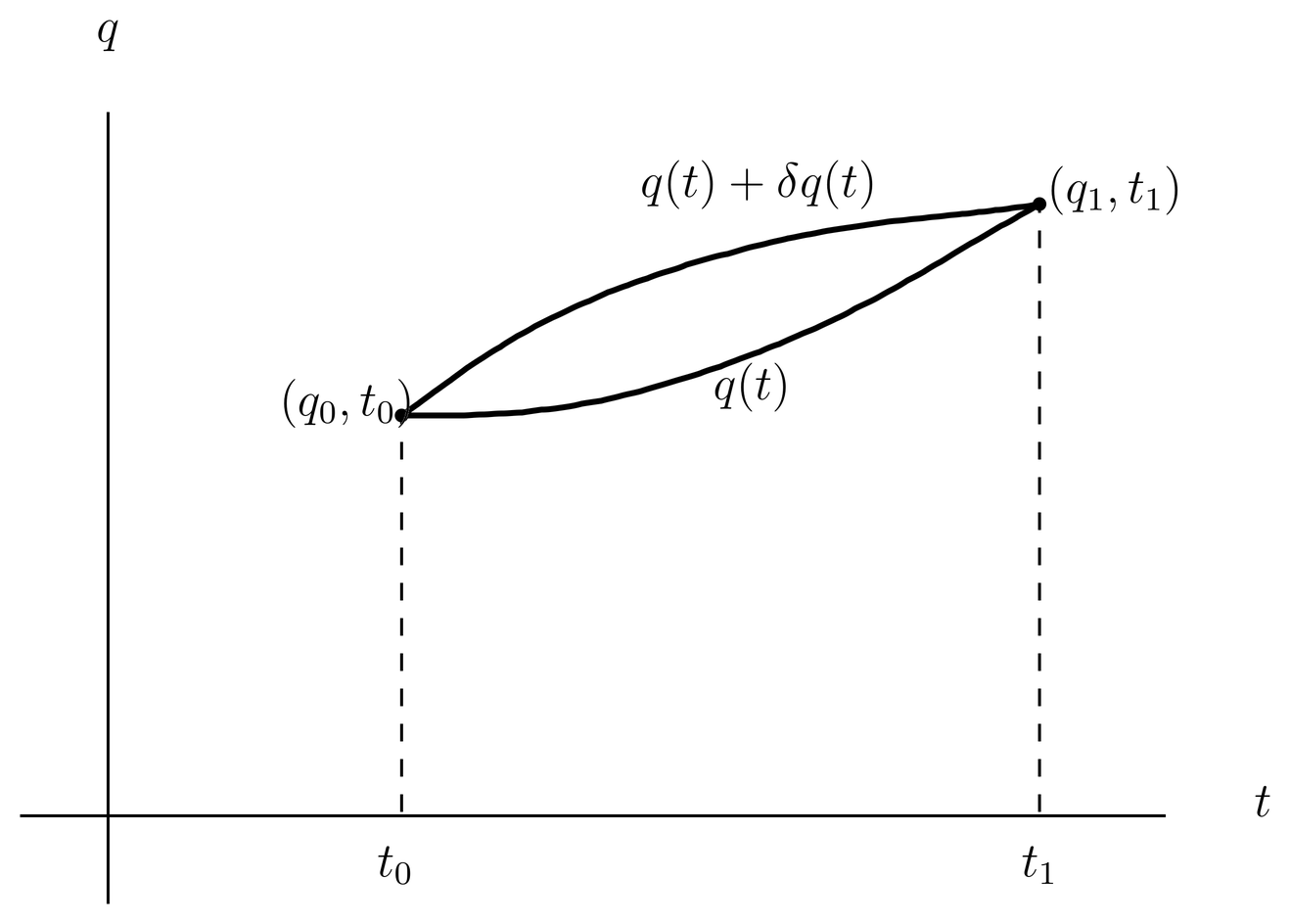
Figure 4:A path satisfying fixed boundary conditions and . Also shown is a modified path , satisfying the same endpoint and endtime conditions.
The Euler-Lagrange Equations
The functional derivative (12) can be computed as follows. Let be any path in the path space, that is, any path satisfying the boundary conditions. It need not be a physical path, that is, one that satisfies Newton’s laws. Let be a small variation that takes the path into a nearby path , as in Figure 4. The new path is also required to be in the path space, so . The velocity along the original path is and that along the modified path is , where
Then the variation in the action is
dropping terms that are second order or higher in . But the second term on the right can be integrated by parts,
where the first major term on the right vanishes because of the boundary conditions . Altogether, we have
Thus by the definition of the functional derivative,
This is the quantity which vanishes along the physical paths, so the equations of motion satisfied by the physical paths are
for . These are the Euler-Lagrange equations.
An ordinary function over some domain may have any number of critical points, from zero to infinity. Similarly, for a given path space, that is, for given values of , , and , the action functional (11) may have any number of critical points. That is, for the given endpoints and endtimes, there may be any number of physical paths, from zero to infinity. Many books erroneously state that the physical path is unique for given endpoints and endtimes.
The Lagrangian, and the Case 
To say that a classical system admits a Lagrangian formulation means that there exists a function such that the Euler-Lagrange equations (19) are equivalent to Newton’s laws. As mentioned, such a formulation exists whenever the system is nondissipative. This is shown by actually finding the Lagrangian function in different cases. We will not go through the proof of equivalence to Newton’s laws here, instead we will just quote the Lagrangian function for the cases of greatest interest to us. The actual proof is straightforward for unconstrained systems, but more elaborate in the case of constraints, especially time-dependent ones.
The most important case for this course is that of nonrelativistic systems in which the forces can be obtained from a scalar potential. Let be the potential energy of the system, expressed as a function of the positions of the particles and possibly the time. It is assumed that there is a force on particle given by
In addition, if there are constraints, then there are also forces of constraint acting on the particles. We do not need to take explicit account of the forces of constraint in a Lagrangian formulation, but they must be dealt with when using Newton’s laws. We assume that the forces (20) and the forces of constraint are the only forces acting on the particles. By using the relations (2), the potential energy can be expressed in terms of the generalized coordinates and possibly the time,
Similarly, by differentiating (2) with respect to time and using the chain rule, the kinetic energy can be expressed as a function of the ’s, the ’s and possibly the time,
where is the mass of particle and where is the number of degrees of freedom.
In this case the Lagrangian is the difference between the kinetic and potential energies,
An important case in practice is that of unconstrained particles interacting by means of electrostatic forces, including “external” electrostatic fields. In this case the potential energy of the particles is
where is the charge of particle and where is the electrostatic potential energy per unit charge due to external fields. The first sum on the right is the electrostatic energy of interaction of the particles among themselves. The sum is taken over all pairs , omitting the diagonal terms which represent the infinite self-energy of the charged particles. The second term is the external potential, corresponding to an external electric field,
Here we use for an arbitrary field point at which the field may be evaluated.
The external potential may depend on time if the charges producing the external fields are moving. Think, for example, of an atom between the plates of a capacitor to which an AC voltage is applied. In this case the external electric field may be written,
where is the amplitude of the electric field, assumed to be pointing in the -direction, and is the frequency. Then the external potential is
The potential (24) only takes into account the interactions of the charged particles in the electrostatic approximation, which is valid for nonrelativistic systems of small spatial extent. That is, the equations of motion are equivalent to
This approximation neglects magnetic effects as well as the effects of retardation and radiation. See 40. The Classical Electromagnetic Field Hamiltonian{} for further discussion.
Magnetic Fields
The Lagrangian formulation may also be applied to problems with magnetic fields. The simplest case is one in which the magnetic fields are external, that is, we ignore any magnetic fields arising from the motion of the charged particles of the system itself. We write the external magnetic field in the form
where is the vector potential. As indicated, the external magnetic field is allowed to depend on time. Then the Lagrangian is
If is given by (24), then the Euler-Lagrange equations are equivalent to
If it is desired to take into account the internal magnetic fields produced by the moving charges of the system itself, this may be done in an approximate way by adding extra terms to obtain the Darwin Lagrangian. See the discussion in Landau and Lifshitz or Jackson. The Darwin Lagrangian has more physics in it than the Lagrangian (30), but it still omits the effects of retardation and radiation. If these are important, one must include the infinite degrees of freedom of the electromagnetic field. See the discussion in 40. The Classical Electromagnetic Field Hamiltonian.
Advantages of Lagrangian Mechanics
The Lagrangian formulation of mechanics affords several advantages compared to Newton’s laws. First, the Lagrangian is a single (scalar) function, which implicitly contains within it all the equations of motion. Thus, if we wish to transform to a new coordinate system, it is much easier to transform the (single, scalar) Lagrangian than the (vector, multicomponent) equations of motion. The Lagrangian formulation is the easiest way to write down the classical equations of motion in curvilinear coordinates.
In addition, if there are constraints, the Lagrangian formulation automatically gives us the correct equations of motion without having to take the forces of constraint into account. This is considerably simpler than working with Newton’s laws, where the forces of constraint must be eliminated.
Third, there is a general relationship in Lagrangian mechanics between symmetries and invariants. That is, every symmetry of the system corresponds to a conservation law. This is called Noether’s theorem.
Finally, the Lagrangian formulation of a classical system leads to the Hamiltonian formulation, which is the point at which we may pass to quantum mechanics.
The main disadvantage of the Lagrangian formulation is that it is unable to account for dissipative effects.
The Momentum
Let us return to the Lagrangian , expressed in terms of generalized coordinates. We define the quantity
which we call the generalized momentum conjugate to . In terms of , the Euler-Lagrange equations (19) can be written,
The physical meaning of the generalized momentum depends on the coordinates used and the nature of the forces.
Consider first Cartesian coordinates, for which we write the momentum conjugate to as (a 3-vector),
Restricting the Lagrangian (30) to a single charged particle interacting with a given (external) electromagnetic field, we find
The first term, , is the usual definition of the momentum in elementary mechanics. We call this term alone the kinetic momentum. In the presence of a nonzero vector potential, however, there is a second term. We call the total momentum of (35) the canonical momentum. The canonical momentum depends on the choice of gauge for the vector potential, so it is not as physical as the kinetic momentum (its value depends on the gauge convention). For this reason one may prefer formulations based on the kinetic momentum. The canonical momentum, however, is necessary for a Hamiltonian formulation of mechanics in the presence of magnetic fields, and it is the canonical momentum that corresponds to the momentum operator in quantum mechanics.
The extra term in the canonical momentum (35) is somewhat mysterious in this formulation of particle mechanics, but it acquires an explanation in terms of the momentum of the electromagnetic field when the field degrees of freedom are included in the system. This is especially simple in the case of Coulomb gauge. This point is discussed further in 40. The Classical Electromagnetic Field Hamiltonian.
In curvilinear coordinates the momentum has other interpretations. For example, consider the case of a particle moving in a potential in 3-dimensional space, for which the Lagrangian in spherical coordinates is
Then the momentum conjugate to the azimuthal angle is
which physically is the -component of the angular momentum , as indicated.
To see how the generalized momentum changes under a change of coordinates, let us temporarily write (with a superscript, that is, a contravariant index) for the coordinates, and let us consider a change of coordinates . See Appendix~\tensor\ for a discussion of contravariant and covariant indices in tensor analysis, and how they transform under coordinate transformations. For simplicity we assume the coordinate transformation is time-independent. Then the generalized velocity transforms according to the chain rule,
which is the transformation law for a contravariant vector. Similarly, the generalized momentum transforms as
that is, as a covariant vector. For example, in spherical coordinates, the generalized momenta are the covariant components of the momentum vector in spherical coordinates.
Taken together, (38) and (39) imply that the quantity , and hence the differential form , are invariants under general coordinate transformations on configuration space.
Regular and Irregular Lagrangians
Expanding out the time derivative in the Euler-Lagrange equations (19), we have
which can be solved for the generalized accelerations if
Lagrangians for which (41) holds are said to be regular. All Lagrangians normally encountered in nonrelativistic particle mechanics are regular, and, in particular, all the nonrelativisitc Lagrangians cited in this Appendix are regular. Irregular Lagrangians do occur, however, in relativistic particle mechanics, and they are common in relativistic field theory, such as in the Lagrangian formulation of the electromagnetic field.
For a regular Lagrangian, we can solve the Euler-Lagrange for the generalized accelerations,
where are some functions. That is, the equations of motion are a system of coupled, second-order differential equations on configuration space. These can be converted into a system of coupled, first-order differential equations by introducing the generalized velocities , and writing,
Lagrangians for Relativistic Problems
Relativistic mechanics can also be put into Lagrangian form. See Appendix~\tensor\ for our notation for relativistic problems (we follow the notation of Jackson, Classical Electrodynamics, 3rd ed).
In a covariant formulation of relativistic mechanics we must not parameterize the particle orbits by time, which is specific to one Lorentz frame. Instead it is desirable to treat the time on the same footing as the three spatial coordinates, and to write for the world line of the particle, where is an arbitrary parameter of the world line. See Figure 5. You might think that proper time would be the natural parameter of the world line, but proper time is linked to the space-time coordinates by the differential relation
and it is desirable to use a parameter that is independent of the coordinates.
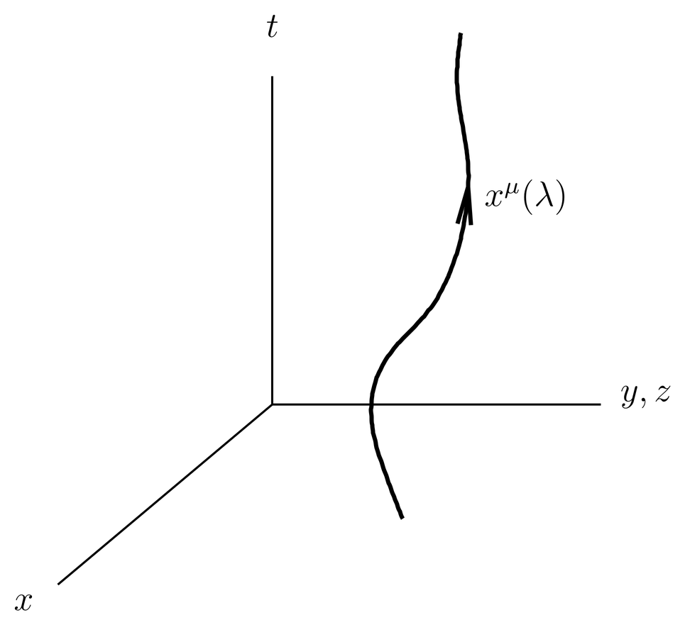
Figure 5:The world line of a particle, where is an arbitrary parameter. One spatial dimension is suppressed in the figure.
which we take to be a function of and . We require the equations of motion to be covariant. This is automatic if the action is a Lorentz scalar, which causes the Euler-Lagrange equations to have the same form in all Lorentz frames. This in turn implies that the Lagrangian must be a Lorentz scalar. This is a powerful constraint on the form of the Lagrangian for relativistic problems that determines it almost uniquely in various situations.
We begin with the case of the free particle. The dynamics of the free particle is invariant under space-time displacements, so the Lagrangian cannot depend on (it cannot depend on our choice of origin of our Lorentz frame). Thus the Lagrangian can depend only on , the world velocity with respect to . The only scalar that can be constructed out of this is
so the Lagrangian must be a function of this quantity. We take it to be
because this makes the momentum conjugate to come out to be the usual 4-momentum of a particle [see (48)]. Notice that with this Lagrangian, , so the action is times the elapsed time as measured by a clock attached to the particle.
The momentum conjugate to is given by a version of (32),
where the time derivatives of our earlier discussion are reinterpreted as -derivatives, and where we use (46). Our use of the lower index on is in accordance with the usual rules for placing indices when we differentiate with respect to something with indices (see Covariant Vectors), and also with the fact that the momentum transforms as a covariant vector [see (39)]. We can raise this index with the metric, obtaining,
and examine the components. The time component is
where is the usual relativistic factor of time dilation,
The spatial components give
where we use the notation explained in The Sign of the Metric, and a Notational Problem for the spatial components of a 4-vector. Equations~(50) and (52) are equivalent to the usual definition of the momentum 4-vector,
where and .
Since the Lagrangian (47) is independent of , the Euler-Lagrange equations are
where again we reinterpret time derivatives [see (19)] as derivatives. After raising the index and multiplying by this becomes
These are the correct equations of motion for the free particle. The parameter has disappeared, as it must, since it was arbitrary.
Now suppose our particle has charge . We wish to incorporate its interaction with an external electromagnetic field, described by the 4-vector potential,
and the field tensor,
The simplest Lorentz scalar we can construct out of and the tensors describing the electromagnetic field is . Other choices such as
will not do, since they vanish. Adding a multiple of to the free particle Lagrangian (47) and adjusting the coefficient to get the correct equations of motion, we find the Lagrangian,
Now the action contains a term,
a relativistic version of an integral related to magnetic flux and gauge transformations (see The Heisenberg and Schr"odinger Pictures are Physically Equivalent).
The new Lagrangian (59) gives the canonical momentum,
We see again the distinction between the canonical momentum (the sum of both terms on the right hand side) and the kinetic momentum (the first term alone). When necessary to distinguish the two momenta, we will write for the kinetic momentum. It is the momentum (without distinction) in the case of a free particle. If we write its components as
where we have raised the index, then the usual relativistic energy-momentum relation is
Notice that this includes the rest mass, so its low velocity limit is .
Now the Euler-Lagrange equations are
or, after raising , using (57), and multiplying by ,
These are the correct covariant equations of motion for a relativistic charged particle in an electromagnetic field. They contain the usual Lorentz force law in their spatial components, and an energy equation in the time component.
Relativistic Lagrangians in -Notation
Sometimes we wish to describe the relativistic dynamics of a particle -notation, that is, with respect to the space and time coordinates and of a specific Lorentz frame. This does not change the fundamental Lorentz covariance of the theory, but it does destroy manifest Lorentz covariance.
It is easy to refer the particle dynamics to the coordinate time of a specific Lorentz frame. Since the parameter of \secrclassmech-13 was arbitrary, we can simply set . Then we have
where . Then the free particle Lagrangian (47) can be written,
Using this to compute the momentum conjugate to , we find
with a minus sign compared to the usual definition of the 3-momentum in relativity theory. This is the same minus sign that we get by replacing by in (48), which leads to . It is another manifestation of the notational difficulties caused by our choice of sign of the metric (see The Sign of the Metric, and a Notational Problem). To make the momentum agree with the usual definition in a -formulation of mechanics we may multiply the Lagrangian by -1. This does not affect the equations of motion.
To include the interaction with an electromagnetic field we set in the interaction term,
so that the entire Lagrangian, including the change of sign, is
Now the canonical momentum is
the relativistic generalization of (35). The canonical momentum is the relativistic version of the kinetic momentum plus the same correction term, , seen in the nonrelativistic formula (35).
It is straightforward to work out the equations of motion that follow from the Lagrangian (70). They are
which are equivalent to the covariant equations (65). The left-hand side is the relativistic definition of the force (the time rate of change of momentum), and the right-hand side is the Lorentz force.
In the low velocity limit we may expand the square root in the first term of the Lagrangian (70). This gives
This agrees with the Lagrangian (30), if we specialize the latter to the case of a single particle and set . There is also the addition of the constant term , which does not affect the equations of motion. Although in the nonrelativistic theory we are accustomed to write the Lagrangian as plus a magnetic term, notice that in the relativistic theory the first term of the Lagrangian (70) is not the kinetic energy, which would be .
Hamilton’s Equations
Let us return to our general discussion of Lagrangian mechanics given in Secs.~\secrclassmech-7--\secrclassmech-12. The condition (41) is also the condition that the definition (32) of the generalized momentum can be solved for the velocities, that is, that we can express the velocities as functions of the ’s, the ’s and the time:
where stands for all the generalized momenta, . Thus for regular Lagrangians we can introduce the ’s as new coordinates, eliminate the ’s from (43), and express the equations of motion as a system of first-order differential equations involving the ’s and the ’s.
The equations of motion can be put into an especially symmetrical form in terms of the Hamiltonian function, defined by
The right-hand side of this expression is a function of , in particular, emerges as a function of due to its definition (32), but we use (74) to eliminate the ’s in favor of the ’s, and express as a function of as shown.
Now we compute , noting carefully that this derivative means holding fixed. We have
where means the derivative of functions (74), taken at fixed . But by (32) the first and third terms on the right of (76) cancel, while the second term on the right can be simplified with the help of (33). The result is . Similarly, we compute , which means holding fixed. We have
where means the derivative of functions (74), taken at fixed . But by (32) the two sums on the right hand side cancel, and we have .
In summary, we find
These are Hamilton’s equations. They are equivalent to the Euler-Lagrange equations in the case of a regular Lagrangian. Hamilton’s equations display a notable symmetry between and .
Examples of Hamiltonians
Let us take a nonrelativistic, unconstrained system of particles interacting by means of a potential , such as the electrostatic potential (24). The kinetic energy is
and the Lagrangian is . The momentum conjugate to is
which can be inverted to solve for as a function of ,
a special case of (74). Then according to (75) the Hamiltonian is
But the first term is twice the kinetic energy, , so altogether,
where we have used (81) to eliminate in favor of . In this example, the Hamiltonian is the sum of the kinetic plus the potential energy, that is, it is the total energy.
Let us take the previous example and add an external magnetic field, producing the Lagrangian (30). Now the canonical momentum is
where we drop the “ext” subscript on . This can be solved for ,
giving another version of (74). Now computing according to (75) and using (85) to eliminate in favor of , we find
We will use this Hamiltonian frequently in this course. It is important to note that the first term is still the kinetic energy, just expressed in a somewhat complicated form because of the use of the canonical momentum (84).
Even in the presence of a magnetic field, the total energy of the system is still the sum of the kinetic and the potential energies. This corresponds to the physical fact that magnetic forces do not change the energy of a particle, because they are always orthogonal to the velocity vector.
The Hamiltonian is the total energy of the system in other examples, too, such as in relativistic problems. More generally, we may define the total energy of the system to be the Hamiltonian. For example, starting with the relativistic Lagrangian (70) and applying the definition of the Hamiltonian (75), we obtain
after taking some effort to eliminate in favor of . The first term is just the kinetic energy of the particle, including the rest mass term , that is, it is , since
Expanding the square root in (87) in the low velocity limit, we obtain
a version of (86) in which the energy includes the rest mass term .
If we attempt to compute the Hamiltonian corresponding to the covariant Lagrangian (47) or (59), we find that it vanishes, . The reason is that these Lagrangians are not regular, and it is not possible to solve for the “velocities” in terms of the momenta . Hamiltonians in the usual sense are generators of translations in time, that is, time measured relative to a specific Lorentz frame. Thus Hamiltonians (in the usual formulation) cannot be covariant. This is one reason why in relativistic quantum field theory there is an effort to get away from Hamiltonians and to shift attention to objects that can support a covariant formulation of the dynamics, such as the Lagrangian, the path integral, and the -matrix.
The Minimal Coupling Prescription
The minimal coupling prescription is a simple rule for passing from a description of a free particle to that of the particle interacting with an electromagnetic field. It can be described as the replacement,
Here the on the left is the momentum (both kinetic and canonical) in the description of the free particle, while on the right is the canonical momentum in the description of the particle interacting with the field. Thus, the entire right hand side is still the kinetic momentum. The replacement takes one expression for the kinetic momentum and replaces it by another. The replacement can be broken into its space and time components, which are equivalent to
Although we have given the minimal coupling prescription in relativistic form, it can be applied to nonrelativistic problems. For example, the energy and momentum of a nonrelativistic free particle are related by
Making the minimal coupling replacement (91), this becomes
which, if we solve for and reinterpret as the Hamiltonian, becomes
a single-particle version of the Hamiltonian (86).
As for a relativistic particle, the energy-momentum relation is
Carrying out the minimal coupling prescription (91) on this and solving for , we obtain the Hamiltonian (87).
The prescription (90) or (91) is called “minimal” because it amounts to using the simplest Lorentz invariant coupling possible between the particle and the electromagnetic field, as explained in \secrclassmech-13. It is just a quick way of getting the Hamiltonian without having to go through the details of the Lagrangian and the Legendre transformation. The Hamiltonian so obtained is classical, but can be taken over into quantum mechanics as a first guess for a quantum description of the system. Minimal coupling does not always give the correct answers from a physical standpoint, that is, sometimes particles interact with the field by means of more complicated couplings than the simplest one. For example, the Hamiltonian (86), interpreted as a quantum Hamiltonian, does not include the interaction of the spin of the particles with a magnetic field (terms that appear in the Pauli equation). But even when the answer is not correct it is still interesting, because any corrections must involve additional Lorentz-invariant couplings that are more complicated than the minimal one.
Although we have only described minimal coupling in terms of particle mechanics, it can also be applied to fields, where it amounts to adding the term
to the field Lagrangian, where is the 4-current associated with the matter field.
Phase Space
The space upon which are coordinates is called phase space. Phase space can be thought of as the state space of the classical system, that is, the space in which a single point represents the dynamical state of the system. The dynamical state of a classical system is the specification of enough information to determine the future evolution of the system. Specifying a point of configuration space (the ’s) is not enough, instead we must also include the velocities (the ’s), or, alternatively, the momenta (the ’s).
A point of phase space represents a complete set of initial conditions because Hamilton’s equations on phase space are first order in time. We can visualize the flow in phase space through the vector field with components , which is called a Hamiltonian vector field. Figure 6 illustrates the Hamiltonian vector field in the 2-dimensional phase space for the harmonic oscillator,
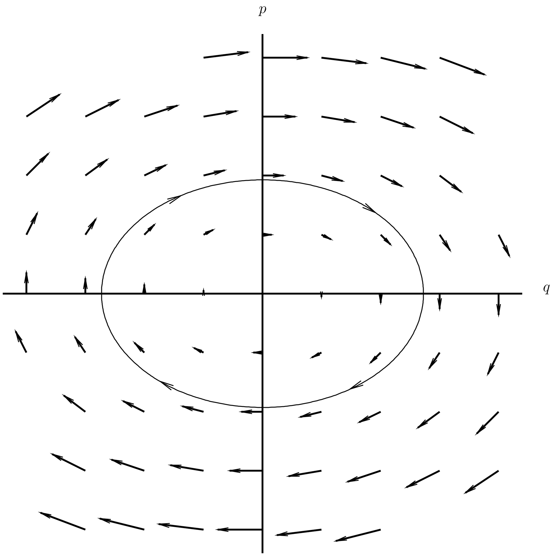
Figure 6:The Hamiltonian vector field in phase space for the harmonic oscillator. One orbit (an ellipse) is shown.
The orbit passing through a point of phase space is obtained by following the arrows of the Hamiltonian vector field. The orbit is tangent to the vector field at each point. One orbit of the harmonic oscillator (an ellipse) is illustrated in Figure 6. Theorems about differential equations guarantee a unique solution , passing through a given initial point at when the vector field is smooth. Thus, there is a unique orbit passing through each point of phase space. Orbits cannot cross one another in phase space, because the interpoint would have two orbits passing through it. Orbits in configuration space, however, are free to cross one another, since the equations of motion on configuration space are second order in time. For example, planets can and do collide.
Time Evolution of Observables
A classical observable is simply any function of , , and possibly . If the observable depends on it is said to have an explicit time-dependence. An example of an explicitly time-dependent observable is the electrostatic potential (27). In addition, any observable has a time-dependence when seen by a particle (or phase point) moving along its orbit, due to the time-dependence of and . This is called an implicit time-dependence. For an observable , the total time derivative as seen by the phase point moving along its orbit is
where we have used Hamilton’s equations (78) in the final form. The first term in (98) represents the explicit time-dependence, while the sum represents the implicit time-dependence.
Conservation of Energy
Setting in (98), we find the rate of change of the Hamiltonian itself along an orbit,
since in that case the sum in (98) vanishes. In particular, if the Hamiltonian has no explicit time-dependence, then , and the Hamiltonian is conserved, . This is the general law of conservation of energy.
The energy (the Hamiltonian) is not conserved if the Hamiltonian has an explicit time-dependence. In practice, such a time-dependence usually arises when a system is interacting with time-dependent, “external” forces, for example, the atom between the capacitor plates that feels the time-dependent electric field (26). Notice in this case that we assume that the external electric field is just a given function of space and time, and we ignore any reaction of the atom back on the charges in the capacitor. In reality, the atom consists of charged particles that produce their own electric field, which has an effect on the external system producing the external electric field. If we include the external charges in our definition of “the system” as well as the back reaction of the atom on these charges, then we have an enlarged system in which energy is conserved.
Similarly, consider a space craft that is obtaining a “gravity boost” by passing close to the planet Jupiter. Because Jupiter is so massive, it is a good approximation to assume that the position of Jupiter is just a given function of time, independent of the position of the spacecraft. Then the spacecraft feels a time-dependent gravitational field due to Jupiter, from which it can extract energy and get expelled from the solar system. In reality, Jupiter does react to the spacecraft, and moves slightly closer to the sun as the spacecraft leaves the solar system. Overall, energy is conserved.
The Poisson Bracket
The final sum in (98) is an example of a Poisson bracket, which is defined in general as follows. Let and be any two classical observables, possibly time-dependent. Then the Poisson bracket of and is another classical observable, given by
In terms of the Poisson bracket, (98) can be written,
The Poisson bracket has the following properties. In the following we use capital letters for classical observables, and lower case letters for numbers (real or complex). First, it is linear in both operands,
Second, it is antisymmetric in the two operands,
Third, it obeys the Leibnitz rule,
Closely related to the Leibnitz rule is the chain rule for Poisson brackets, which is the following. If observable depends on a collection of other observables, say,
then
A similar expression holds when depends on further observables.
Fourth, it satisfies the Jacobi identity,
All these properties are straightforward to prove from the definition.
The Poisson brackets of the phase space coordinates, the ’s and ’s, among themselves are notable. These are
Conserved Quantities
In general, a conserved quantity or constant of the motion is a classical observable that is constant as we follow the Hamiltonian flow along an orbit. That is, is a constant of motion if
A time-independent constant of the motion is one with no explicit time-dependence, so that . It follows that time-independent constants of the motion are classical observables whose Poisson bracket with the Hamiltonian vanishes, . As we say, such observables Poisson commute with the Hamiltonian.
In particular, the Hamiltonian Poisson commutes with itself, , due to the antisymmetry of the Poisson bracket, property (103). Thus we recover (99).
Liouville’s Theorem
Liouville’s theorem states that the volume of a region of phase space is constant in time, when the boundary of that volume and all the points inside it are allowed to move down their respective orbits by the same amount of elapsed time. In systems of one degree of freedom, in which phase space is the 2-dimensional - plane, Liouville’s theorem implies conservation of area, as illustrated in Figure 7.
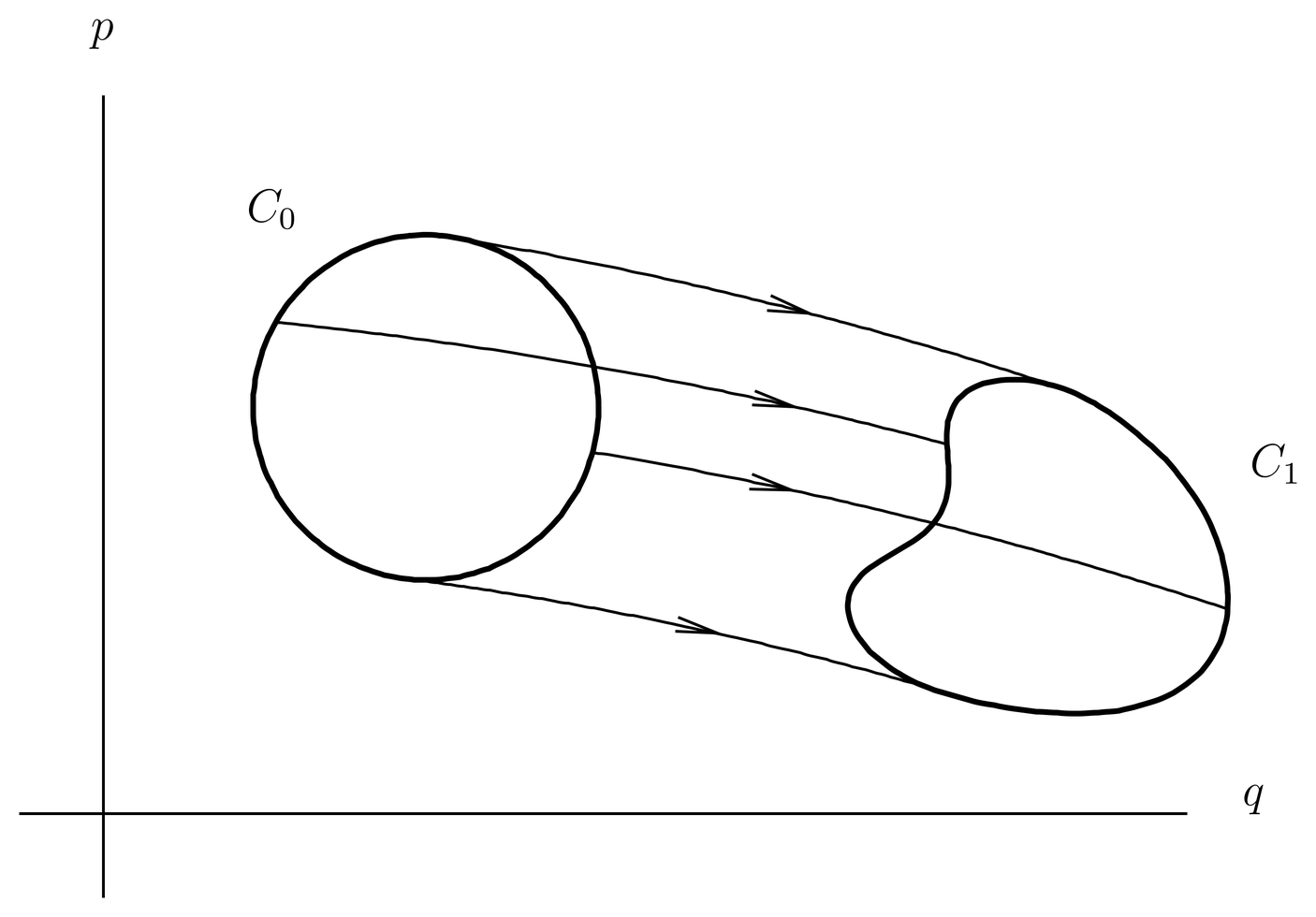
Figure 7:Liouville’s theorem in the phase plane. All points on the boundary of curve are allow to follow the Hamiltonian flow for the same amount of elapsed time, thereby mapping into . The area enclosed is constant.
Liouville’s theorem is proved by a -dimensional version of Gauss’s law. The essence of the proof is the vanishing of the total divergence of the flow vector in phase space,
Classical Statistical Mechanics
A classical system whose state is only known statistically may be described at a certain time by means of a probability distribution on phase space. In general changes in time, so is a function of , and . The normalization condition is
for all . Alternatively, we may interpret as giving the density (per unit volume in phase space) of an ensemble of systems, each of which is governed by the same Hamiltonian . The systems do not interact with one another. In this interpretation, the integral of over all phase space is the number of systems in the ensemble. It differs from the previous interpretation only in the normalization of .
The evolution equation for may be obtained as follows. Consider an infinitesimal volume of phase space, with a certain number of systems of the ensemble in it. Let the volume move with the Hamiltonian flow, as in Figure 7. The volume of the volume element does not change in this process, according to Liouville’s theorem. Nor does the number of systems in the volume element, since the individual systems just evolve according to the (common) Hamiltonian. Therefore the number of systems per unit volume, which is , is constant as we move along orbits. That is,
This is the Liouville equation.
Let be time-independent. It follows from the Liouville equation that the probability density can be constant in time (that is, ) only if . The only way this can happen is if is a function of the time-independent constants of the motion. That is, let , where the ’s are time-independent constants of the motion. Then by the chain rule property (106) of the Poisson bracket we have
To analyze these statements carefully requires ergodic theory, which we will not go into.
In some cases the only time-independent constant of the motion is the Hamiltonian itself. Then is constant in time only if is a function of the Hamiltonian. Two cases are of interest. One is
where is a normalization constant and is an energy. The ensemble consists of systems of a known energy . This is called the microcanonical ensemble. It is appropriate for isolated systems, in which the energy is constant.
Another important case is
where is the usual thermodynamic parameter ( is the Boltzmann constant, and the temperature). This is the canonical ensemble, appropriate for a system in contact with a heat bath at temperature . Here is the normalization of , so that
The quantity is the (classical) partition function.
Hamilton’s Principal Function
Let us return to the action functional (11), which is defined on paths belonging to the path space defined by (13). This path space is parameterized by the endpoints and and the endtimes and . As noted, there may be more than one physical path in this path space, that is, more than one path on which the action is stationary. Let us denote these physical paths by , where is a “branch” index labeling the paths. Generally the branch index is discrete, so we can take .
The physical paths cause the action to be stationary. Does the action play any other role in mechanics? In particular, is there any significance to the value of the action functional, evaluated on a physical path? This value depends only on the branch index, and on the parameters of the path space itself. We will write for this function, so that
This function is called Hamilton’s principal function. It is also called “the action,” but you must not confuse it with the action functional or the other quantities called “the action” in classical mechanics. (They all have dimensions of action, but otherwise are different.)
Hamilton found that his principal function satisfies some interesting differential equations, which imply that knowledge of this function is equivalent to knowing the general solution of the classical equations of motion. This is remarkable, because Hamilton’s principal function is a single function, while the general solution of the equations of motion involves functions, giving the final , coordinates as functions of the initial , coordinates and the time.
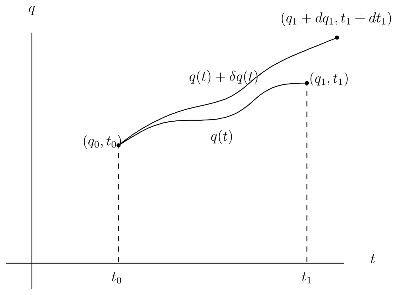
Figure 8:A path satisfying fixed boundary conditions and . Also shown is a modified path , satisfying the same endpoint and endtime conditions.
Figure 8 illustrates a physical orbit in the - plane and a nearby physical orbit , whose final position and have been shifted slightly by amounts and . That is, the modified orbit satisfies
This is at the upper limit. As shown in Figure 8, the modified orbit coincides with the original orbit at the lower limit, that is,
so .
Figure 8 differs from Figure 4 in several respects. First, the path in Figure 4 is any path satisfying the endpoint and endtime conditions (13), generally a nonphysical path, while in Figure 8 is a physical path. That is, in Figure 8 is one of the paths mentioned above, but we have suppressed the index. Next, in Figure 4 is a variation about the generally nonphysical path , producing another, generally nonphysical path, in the same path space specified by (13). In Figure 8, however, is the difference between two physical paths, and . Also, the modified path belongs to a different path space than , that is, it satisfies the modified endpoint and endtime conditions (118) at the upper limit.
With these understandings, we can compute the difference in Hamilton’s principal function between the two paths of Figure 8. We suppress the branch index on as well as on . We have
where and where we have expanded the right hand side out to first order in small quantities. We integrate the last term by parts as we did in (16), to obtain
This time, however, does not vanish at , while the integral on the right does vanish because the physical path satisfies the Euler-Lagrange equations. The result is simply
where means the momentum of the path , evaluated at . Putting this back into (118), we have
Now expanding (118) out to first order in small quantities, we have
which can be solved for . Substituting this into (125) gives
where
is the Hamiltonian, evaluated at the endpoint of the path .
(127) implies
In Figure 8 we have varied the upper endpoint and endtime of the physical path , while keeping the lower endpoint and endtime fixed. If we also vary the lower endpoint and endtime, we find
The Hamilton-Jacobi Equation
Hamilton realized that (129) and (130) allow the general solution of the equations of motion to be obtained once his principal function is known. Since is a function of the parameters of the path space, , the -derivative in (130) gives the initial momentum as a function of these parameters,
where we just write for the vector of initial momenta , . This equation can be solved for , giving us functions,
where is the value of the function . The function gives the final position as a function of the initial position and momentum and the initial and final times and .
Similarly, the -derivative of (129) gives the final momentum as a functions of the parameters of the path space,
But by substituting (132) into this, we can eliminate and express as a function of :
in which is the value of the function . The function gives the final momentum as a function of the initial position and momentum and the initial and final times and .
Taken together, the functions and constitute the general solution of the equations of motion, that is, these functions specify the final dynamical state given the initial dynamical state and the two times. Given Hamilton’s principal function , the derivation only involves differentiations and algebraic operations (inverting systems of equations). There are no differential equations to be solved.
Thus we would like to find a way of determining Hamilton’s principal function . This function is defined in (117) as the integral of the Lagrangian along the orbit, but if the orbits are not known we cannot do the integral. Therefore we seek an equation satisfied by .
The desired equation comes from the time derivative in (129). In that equation, means the Hamiltonian evaluated at the final point on the orbit, that is, it is . At that point, however, is given by the -derivative in (129). Putting the pieces together, we have
This is the Hamilton-Jacobi equation for the function . It determines the and dependence of . To determine the and dependence, we treat (130) in a similar manner. This gives
in effect a second Hamilton-Jacobi equation also satisfied by . The solution of the classical equations of motion (Hamilton’s equations), a system of coupled, ordinary differential equations, is equivalent to the solution of the pair of partial differential equations, (135) and (136).
Solving (135) and (136) for Hamilton’s principal function is not usually a practical way of solving the equations of motion of classical mechanics. There is a modification of this procedure, however, due to Jacobi, that is quite useful in certain applications. For the case of time-independent Hamiltonians, Jacobi’s theory leads to another version of the Hamilton-Jacobi equation,
where is an energy. This can be regarded as a time-independent version of the Hamilton-Jacobi equation. Here is a function of and a collection of parameters which turn out to be constants of motion. We will not pursue this topic here, which is covered in advanced books on classical mechanics. But Hamilton’s principal function is important in semiclassical treatments of quantum mechanics (see 07. The WKB Method\ and \pathint), where it appears as the phase of the propagator. If one must evaluate it, the easiest way is usually to use the definition (117). The function also appears in semiclassical treatments of quantum mechanics, where it is essentially the phase of an energy eigenfunction.
Canonical Transformations
Coordinate transformations on phase space are used for many purposes. Classical perturbation theory, for example, is based on the idea of applying successive coordinate transformations that simplify the equations of motion to progressively higher powers of the perturbation parameter. When a coordinate transformation is carried out, a question is whether the new equations of motion can be written in the standard Hamiltonian form (78).
Let be the old coordinates on phase space and let and stand for invertible functions of that represent a new coordinate system on phase space. That is, let
where, as indicated, the coordinate transformation is allowed to depend on time. Suppose now that for all old Hamiltonians there exists a “new Hamiltonian,” call it , such that the new equations of motion are given by
Then it can be shown that the new coordinates and satisfy the Poisson bracket relations,
In other words, the new coordinates satisfy the same Poisson bracket relations among themselves as the old coordinates. See (108).
Conversely, suppose the coordinate transformation satisfies (140). Then it can be shown that a new Hamiltonian exists such that the new equations of motion are (139).
A coordinate transformation that satisfies (140) is called a canonical transformation. Canonical transformations are conveniently specified in terms of scalar “generating functions,” of which Hamilton’s principal function and the function of (137) are examples. There is also the problem of determining the new Hamiltonian , given a canonical transformation and an old Hamiltonian . If the transformation is time-independent, then the new Hamiltonian is the same as the old one, just transformed to the new coordinates. That is, in this case. In the general, time-dependent, case, is not the same as , rather there is an extra term involving the generating function. These topics are covered in advanced courses on classical mechanics.