02. The Postulates of Quantum Mechanics
Introduction
In these notes we present the postulates of quantum mechanics, which allow one to connect experimental results with the mathematical formalism described in 01. The Mathematical Formalism of Quantum Mechanics. Actually, we are not ready to state the postulates in their complete and final form, since that requires the use of the density operator, which we discuss in 03. The Density Operator. Therefore our first version of the postulates will involve some undefined terminology, and will be incomplete. Nevertheless, even in their incomplete form, the postulates explain a good deal about the mathematical formalism of quantum mechanics and its relation to physical reality.
These postulates are not supposed to be obvious. In fact, even after the correct equations describing quantum mechanics had been discovered (by Heisenberg and Schr"odinger, in 1925--1926), it was still not obvious what the correct interpretation should be. The interpretation presented in these notes and the next set is the orthodox one, although there are controversial aspects about it and there are alternatives that are active competitors even today. For example, recent work in cosmology has led to renewed interest in the “many worlds” interpretation, in which the “wave function of the universe” plays a role. For now it is best to state the postulates of the orthodox interpretation and see how they work out on some specific physical examples.
Postulates of Quantum Mechanics (Incomplete Form)
In their incomplete form, the postulates of quantum mechanics are the following:
1. Every physical system is associated with a Hilbert space . We call the vectors of this space kets.
2. Every pure state of a physical system is associated with a definite ray in . We postpone for a while the definition of a pure state, but a ray was defined in (9). In practice we often represent the state of a system by some nonzero ket lying in the ray in question. In this course we will often refer to a nonzero ket as the “state” of the system, but really it is the ray that corresponds to the state (the normalization and phase of the ket are of no physical significance).
3. Every measurement that can be carried out on the system corresponds to a complete Hermitian operator (an observable).
4. The possible results of the measurement are the eigenvalues of , either the discrete eigenvalues or the continuous ones .
5. In the discrete case, the probability of measuring is
where is the projection operator onto the eigenspace corresponding to eigenvalue , as indicated by (128), and where is any nonzero ket in the ray representing the state of the system. In the continuous case, the probability of measuring to lie in some interval of the continuous spectrum is
where is the projection operator corresponding to interval , as in (132). Notice that the probabilities in (1) and (2) depend only on the ray, not on which ket is chosen to represent the ray.
6. After a measurement with discrete outcome , the system is represented by the ket , where represents the system before the measurement. Note that in this case, the system is in an eigenstate of with eigenvalue after the measurement. In the continuous case, with outcome , the system is represented by after the measurement, where again is as in (132).
As postulate~5 shows, the predictions made by quantum mechanics are of a statistical nature. The probabilities referred to in that postulate are determined experimentally by repeating the same measurement on a large number of identically prepared systems. The fact that identically prepared systems can yield different results on successive measurements is a point that we will discuss after we give some examples.
We emphasize that quantum mechanics makes statistical predictions about measurements on an ensemble, that is, a collection of (conceptually) an infinite number of identically prepared systems. Although we often use language like “the wave function of the electron,” in reality the state vector (or wave function) does not describe an individual system, but only the statistics of an ensemble. And postulate~6, also called the collapse postulate, does not refer to the “collapse” of any individual system, but rather the creation of a new ensemble, described by a new state vector, that results from the act of making a measurement on the old ensemble.
There is a seventh postulate, not listed here, which states that the state vector evolves in time by means of a time-dependent, unitary transformation. This subject will be taken up in 05. Time Evolution in Quantum Mechanics. Postulate~7 is actually in conflict with postulate~6, assuming that the measuring apparatus is governed by the same rules of quantum mechanics as the system being measured. This is because the projection required by postulate~6 cannot be achieved by unitary transformations, nor can the measurement apparatus end up in a definite state (indicating the result of the measurement) by such means. Much of the ongoing discussion and debate regarding the quantum theory of measurement involves such issues as these in an attempt to explain how in practice we do end up with definite measurements. An aspect that cannot be neglected is that a real measurement apparatus is always macroscopic object that cannot be isolated from its environment. Thus any consideration of the quantum state of the apparatus must take into account the interactions with the environment in some statistical way.
We could pursue these questions but for now the more important task is to see how these postulates actually work in practice. For example, we will have to answer questions such as the following: How do we know what Hilbert space is associated with a given physical system? What operator corresponds to definite measurements? And which ray corresponds to a definite (pure) state of system?
Postulates Applied to the Stern-Gerlach Experiment
To answer such questions, we will analyze the Stern-Gerlach experiment, pretending that we know nothing except the experimental results and the postulates listed above. In particular, we will pretend that we know nothing about wave functions, spin, Pauli matrices, the Schr"odinger equation, etc. The following presentation is based closely on that given by J. J. Sakurai, Modern Quantum Mechanics.
Suppose we are working with a beam of silver atoms, as in the original Stern-Gerlach experiment. From a modern perspective, we know that silver atoms possess a magnetic moment because of their single unpaired valence electron, so that the measured value of any component of magnetic moment is , where is a Bohr magneton (this is in Gaussian units; see Appendix~\emunits). The silver atom has the same electronic spin and magnetic moment as a free electron, but it is electrically neutral. Charged particles are not suitable for a Stern-Gerlach experiment, because in practice the ordinary Lorentz force is much larger than the force due to the magnetic moment, . The original experiment of Stern and Gerlach in 1921 provided a measurement of , with a result in good agreement with Bohr’s value. We also know that the magnetic moment operator is proportional to the spin operator, , where any component of spin takes on the values . In the following discussion, however, we will play dumb and ignore all of this, and instead we will work solely with the experimental results. For the same reason, we will speak in terms of measurements of magnetic moment, not spin.

Figure 1:A beam of silver atoms is subjected to a measurement of , after which the atoms with are passed to a second magnet which measures .
Consider the tandem Stern-Gerlach apparatus illustrated in Figure 1, in which we first measure the -component of the magnetic moment , and then pass the beam with to a second magnet which measures . The experimental result is that the two beams emerging from the second magnet, with , each carry 50% of the atoms that entered that magnet.
Since a measurement of gives rise to two possible outcomes, we must assume according to postulates~3 and 4 that the operator has two possible eigenvalues, . The same is true for and , or indeed, for any component of spin (in any direction). Therefore the Hilbert space must be at least 2-dimensional, since the eigenspaces corresponding to are orthogonal. Indeed, measurements of the components of the magnetic moment alone give us no indication that the Hilbert space has more than two dimensions. The easiest way to proceed with the following argument is simply to assume that the eigenvalues are nondegenerate, and then to come back later to the question of degeneracies. Under this assumption, the eigenspaces are 1-dimensional, the ket space has exactly two dimensions, and it is spanned by the eigenkets of with eigenvalues . It is also spanned by eigenkets of or with eigenvalues , and therefore the pair of eigenkets of any one of these operators must be expressible as linear combinations of the eigenkets of any other operator.
Let us denote some normalized eigenvector of with eigenvalue by ; we say “some” because any other vector differing from this one by an overall phase would work just as well at this stage of the argument. Similarly, let us choose normalized eigenvectors , , and (we will henceforth omit the specification in the eigenkets of this operator). Because eigenkets corresponding to distinct eigenvalues are orthogonal, we have
In accordance with postulate~2, the state of the atomic beam at various stages in the apparatus is described by some state vector (as we will discuss later, the spin system is in a pure state anywhere after the measurement of in the first magnet). Also, according to postulate~6, after the measurement of with result , the state of the system is specified by , as indicated by the ket attached to the upper beam in Figure 1. This is because by our assumption the eigenspace of with eigenvalue is one-dimensional, that is, it is a ray, so the projection operator onto this subspace produces a vector in that ray. The state of the system is determined by the ray, which is specified by any nonzero vector that lies in it, such as . Similarly, the two beams emerging from the second magnet, which measures , are represented by the state vectors . We represent the state entering the second magnet as a linear combination of the eigenkets ,
where are the expansion coefficients. Since and are orthogonal, this implies
Then, according to postulate~5, we have
where
is the projection operator onto the eigenspace of . The denominator in (2) is unity because is normalized. Therefore (6) becomes
where we use (4) and the experimentally measured probability. This implies
where is an unknown phase factor. But since is also , a similar argument gives
where is another unknown phase. Thus, we have

Figure 2:Same as Figure 1, except the beam with is fed into the second magnet.
In general, the wave function of a system is the expansion coefficients of the state vector with respect to some specified basis. Since the coefficients and are the expansion coefficients of with respect to the eigenbasis of , they constitute the wave function in the -representation. We see that the analysis so far, which makes use of the measured probabilities in Figure 1, has determined the wave function only to within the two phases shown in (11). We will now pin down these phases by using a combination of further experimental data and phase conventions.
(11) can be simplified by changing the phase of the ket so as to absorb the phase on the right hand side. Let and multiply (11) by , setting . Then we have
after dropping the primes. Now we have established a phase convention for the ket and we cannot change its phase again. By a similar analysis, if we feed the beam emerging from the first magnet with into the second magnet, as illustrated in Figure 2, and analyze the probabilities exactly as we have done here, we obtain
where is another phase. Now we have fixed the phases of both kets .
But the phases and are related, for by orthogonality we have
or . Thus, (12) and (13) can be written
Similarly, suppose we measure instead of in the first magnet in Figs.~Figure 1 and Figure 2. Then the two beams that emerge from the second magnet still carry 50% each of the silver atoms, and an analysis just like that presented above gives
where is another phase. Now the phases of kets have been fixed.
We can now write down the operators representing the components of in the basis. For example, according to (131) we have
which can be transformed to the basis by substituting (15). This gives
Similarly, we find
and of course we have
Next, a relation can be found between the phases and by imagining another Stern-Gerlach experiment, like Figure 1 except that we measure in the second magnet instead of . Again, we can take it as an experimental result that the two values are measured with equal probability. Therefore we have
where we use (15) and (16). But this implies , or
Thus, the two unknown phases in (18) and (19) reduce to one unknown phase and an unknown sign.
The remaining unknown phase, say, , can be pinned down by choosing a phase convention for the ket ; for example, we can make the matrix elements of either or in the basis purely real, but not both, because by (22), if the matrix elements of one of these operators is real, those of the other operator must be purely imaginary. We see that it is impossible to satisfy the postulates of quantum mechanics and the experimental results with only real numbers; complex numbers are necessary. Here we choose to absorb the phase into the definition of the ket , so that (18), (19) and (20) become
We notice that we cannot change the phase of without messing up equations such as (15) or (16). Thus, all the freedom in phase conventions has been used up. To state results equivalent to (25), we can write out the matrices representing the three operators in the basis,
where the basis vectors are ordered , . We frequently write equations like (26), but we do not really mean that the operator on the left is equal to the matrix on the right, instead we mean that its matrix elements in some given or understood basis are given by the matrices. Here the basis is the eigenbasis of . We see in (26) the appearance of the Pauli matrices.
We see that to within a final unknown sign, the three Pauli matrices are determined solely from the postulates of quantum mechanics, the experimental results, and some phase conventions. But there is the question of the final, unknown sign. Sakurai has some discussion of this point, but he never definitively settles the issue. We will look at this question more carefully in Prob.~\prbrpostulat-2.
Compatible or Commuting Observables
So far we have simply assumed that the eigenspaces of (and , ) are nondegenerate. How would we know if this were not true? If we were given a Hermitian operator or matrix as a purely mathematical problem, then the answer could be obtained purely by mathematics: we first compute the eigenvalues, and then the order of the degeneracy of an eigenvalue is the number of linearly independent eigenvectors of that eigenvalue. But here we are building up the Hilbert space out of the results of physical measurements, and there must be physical meaning to any degeneracies that might exist. As we will now show, the answer to this question involves the notion of compatible or commuting observables.
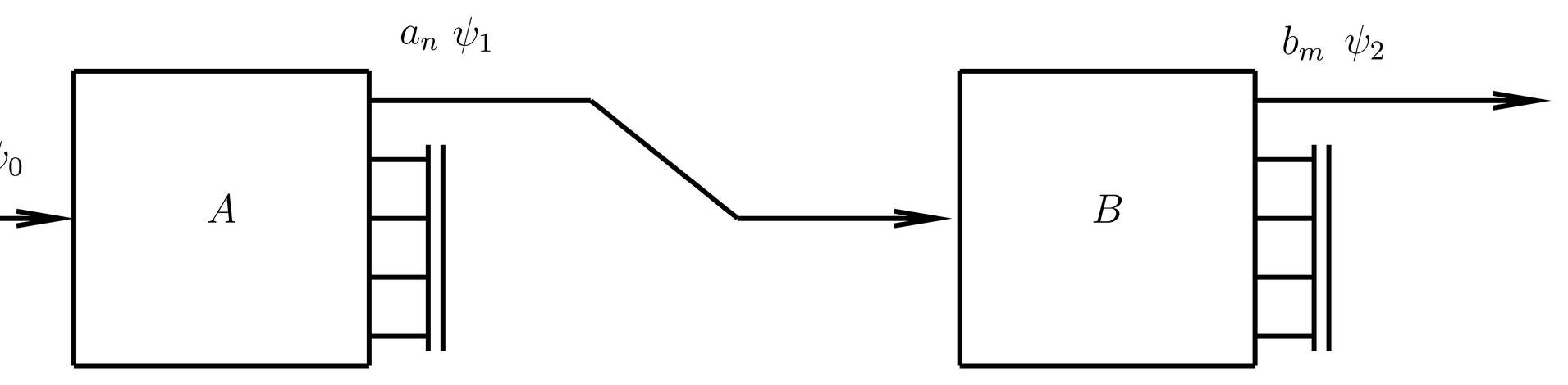
Figure 3:A quantum system is subjected to a measurement of two observables, first , and then .
Consider an idealized measurement such as illustrated in Figure 3. A system that is known to be in a pure state is first subjected to a measurement of observable . Out of the several possible outcomes, all are thrown away except . The system after the measurement of is described by ; this system is passed to a device that measures observable , and all outcomes except are thrown away. The state of the system after the second measurement is described by .
According to the postulates, the probability of measuring in the first apparatus is
where is the projection operator onto the eigenspace of corresponding to eigenvalue . Also, the ket describing the state that emerges from the first filter is
Next let us compute the probability of measuring first and then . This is the (conditional) probability of measuring given that we had , multiplied times the probability of measuring in the first place. We denote the probability of this compound measurement by ; it is given by
where is the projection operator onto the eigenspace of with eigenvalue . But we also have
where we have used (28) and the fact that is Hermitian and idempotent. Thus, the denominator of the first factor in (29) cancels the numerator of the second factor, and we have
Similarly, if we reverse the order of the measurements, measuring first and next , we obtain the probability
These two probabilities are not equal, in general.
Now it can be shown that if , then , so in this case we have
so that both probabilities are equal,
Conversely, it can be shown that if the probabilities and are equal for all initial states and all and , then .
Altogether, we see that probability of a compound measurement is independent of the order of the measurements, for all initial states and all outcomes of the two measurements, if and only if the observables commute. This is the physical meaning of commuting observables. Commuting observables are also said to be compatible. A lesson of this analysis is that it is in principle an experimental matter to determine if two observables, corresponding to definite measurement processes, commute; we simply carry out those measurements in different orders on a large number of systems, and compare the resulting probabilities.
We have described an example of what we might call quantum statistics, in which probabilities depend on the order in which measurements are carried out. A similar problem in classical statistics, by which we mean ordinary statistics, is the following. Suppose we have an urn containing balls with spots of various colors painted on them. If we first select the balls that have a red spot, and then feed these to a device that selects balls that have a green spot, then what comes out is the set of balls that have both a red and a green spot. The number of these balls, divided by the total number of balls in the urn, is the probability of selecting a ball with both a red and a green spot from the urn in the first place. Moreover, the same number is obtained if we select balls with green spots first and then those with red spots. The order does not matter. In this sense, classical statistics is commutative, while quantum statistics is noncommutative. We will have more to say later about the dependence in quantum mechanics of experimental results on the order in which measurements are carried out.
Resolving Degeneracies; Complete Sets of Commuting Observables
Let us now return to the question of degeneracies. Referring to Figure 3, how do we know if the eigenvalues of the operator are degenerate? (You may wish to review the proof of the theorem that commuting observables possess a simultaneous eigenbasis, given in Simultaneous Eigenbases of Commuting Observables, to better understand this .) If an eigenvalue is degenerate, then the eigenspace corresponding to this eigenvalue is multidimensional, so we are asking about the dimensionality of the subspaces . The answer is obtained by searching for other observables that commute with , to see if one of them will `resolve’ the degeneracy of , that is, produce more than one outcome when a measurement of is made subsequent to the measurement . If such an observable can be found, then the states emerging from the -apparatus lie in the simultaneous eigenspaces of the operators and , which are subspaces of the eigenspace of . A vector lying in one of these subspaces is obtained by applying the projectors and (in either order, since they commute) to an arbitrary ket, such as in the figure. In this case, the order of the degeneracy of is at least equal to the number of outcomes of the subsequent -measurement, since each of the simultaneous eigenspaces is at least one-dimensional.
However, these simultaneous eigenspaces of and may themselves be degenerate. To find out if they are, we can search for another operator that commutes with both and , that will resolve the simultaneous eigenspaces of and into smaller subspaces. The process continues until no more resolutions are possible; then the set of observables constitutes a complete set of commuting observables, or CSCO for short. At this point we can declare that the simultaneous eigenspaces of the CSCO are nondegenerate, and the dimensionalities of all simultaneous eigenspaces of all operators in the CSCO are determined.
Once we have found a CSCO, then any new observable that commutes with the CSCO must be a function of the members of the CSCO. This is because the new observable does not produce any further resolutions of the simultaneous eigenspaces of the CSCO, so its eigenvalue on any one of these (one-dimensional) subspaces is just a number that can be regarded as a function of the eigenvalues of the members of the CSCO. This is what we mean by a function of an operator (see A Function of an Observable).
How do we know if we have gone far enough in the search for operators when trying to construct a CSCO? In short, we don’t. If we cannot find a new operator (that is, a new measurement process) that commutes with the operators already in the list and that creates a further resolution of the eigenspaces, it may be due to the lack of such an operator, or the lack of our imagination in searching for one. In practice, this means that there are degrees of freedom that we are ignoring, either because we don’t know about them or because they are not important for the physics we are interested in. For example, in the usual discussion of the hydrogen atom we ignore the degrees of freedom associated with the quarks in the nucleus.
In other words, we often choose not to go all the way to a complete set of commuting observables because we are only interested in some subset of the degrees of freedom of a system. For example, in our discussions of the Stern-Gerlach apparatus, we have been ignoring the spatial degrees of freedom of the silver atom, as well as the internal degrees of freedom representing the motion of the electrons around the nucleus, the motion of the nucleons in the nucleus, the quarks in the nucleons, etc. If we were to include the spatial degrees of freedom of the silver atoms as well as the spin, our Hilbert space would be infinite-dimensional (actually, ).
For another example, we frequently treat electrons as spinless particles (effectively ignoring the spin degrees of freedom), so that the wave function is a scalar instead of a 2-component spinor. This is physically justified in the common case that the electron is moving in an electrostatic field, since spins do not interact with electric fields. It may also be useful as an approximation when spin-dependent effects are small, as they usually are in nonrelativistic quantum mechanics. Later, if we incorporate spin in a more realistic model, we will find that the Hilbert space becomes enlarged and new quantum numbers appear.
Noncommuting Measurements
As discussed above, it is a feature of quantum mechanics that the outcome of measurements depends in general on the order in which they are taken. This is sometimes described by saying that when we measure one observable, we introduce an unavoidable and uncontrollable disturbance in the values of all other observables that do not commute with the one we are measuring. For example, when measuring , we disturb the values of and , or when measuring the position of a particle we disturb its momentum. In comparison to the filtering of classical ensembles, for example, selecting balls from an urn with different colored spots on them, it is as if when we select a ball and discover it has a red spot, this fact alone causes all the other spots on the ball to be replaced by new ones with randomly chosen colors.
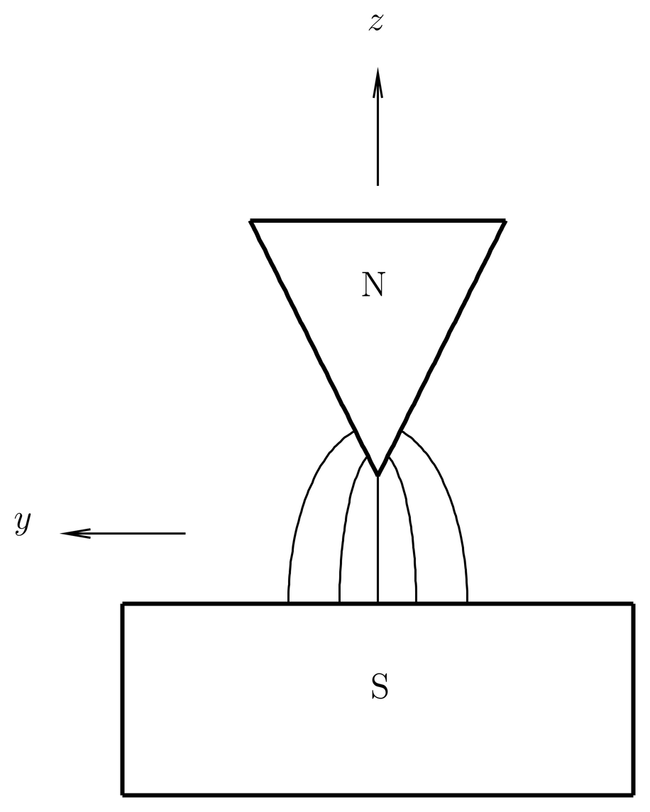
Figure 4:The Stern-Gerlach apparatus seen from one end.
Such disturbances in noncommuting variables also occur in classical mechanics, it is just that in the classical framework we can in principle reduce the disturbance to an arbitrarily small value. To understand this point, let us consider the measurement of in a Stern-Gerlach apparatus in more detail, adopting a classical point of view. Measuring the force on an object in an inhomogeneous magnetic field in order to measure its magnetic moment is something we can do with any magnetized object, including macroscopic ones for which classical mechanics is valid.
An end-view of the apparatus is sketched in Figure 4. The beam is directed along the -axis and runs just below the knife edge of the upper pole tip, where the magnetic field has the largest gradient. The force on the atoms is small, so the magnet extends as far as practicable in the -direction, to maximize the momentum transfer in the -direction. Obviously this momentum transfer must be greater than the statistical spread in the beam in in order to see the effect at all. Assuming the beam is of small spatial extent, we can assume the magnetic field is purely in the -direction at the location of the beam (directly below the pole tip), , so at the location of the beam. Actually, ignoring fringe fields, everywhere due to symmetry. Both the - and -components of have nonzero gradients, however, at the location of the beam (these gradients are restricted by ). The force is . The magnetic moment characterizes the magnetic particle and is a function of time, but it does not depend on space so the force can be written
The magnetic moment itself is not constant in the magnetic field, but precesses according to
where is in the direction of . For the silver atom, has the magnitude
(36) applies to a silver atom, but would not be true for a macroscopic magnetized object unless the magnetic moment were proportional to the angular momentum which is assumed to be large. Otherwise a more complicated equation of motion for must be used. Of course Stern and Gerlach did not know this about silver atoms, but for simplicity we will content ourselves with the simple equation of motion (36), which is correct for silver atoms.
The consequence of (36) is that precesses about the direction with frequency , sweeping out a cone, so that its component along (in this case, ) is constant, while the component of perpendicular to rotates in a circle with frequency . In fact, in a real Stern-Gerlach experiment, the atom stays in the magnetic field for a time that is much greater than the precession period . This is because, as mentioned, it is desirable to keep the particle in the inhomogeneous magnetic field as long as possible to maximize the momentum transfer.
Due to the precession, the component in (35) averages to zero on time scales long compared to the precession time, and the average force felt by the particle is
where we use the fact that near the pole tip the gradient of is predominantly in the -direction. Thus, the momentum transfer in the -direction is
assuming does not change much as the beam gradually bends in response to the force (that is, assuming the spatial displacement in the -direction is small enough, something that may or may not be true in practice).
An important point of this analysis is that while we do measure the (constant) value of while the atom is in the inhomogeneous magnetic field, the other two components and undergo precession and so are not constant. This happens even in a classical description, and is an example of the fact that measuring an observable introduces a disturbance in other observables that do not commute with it. In classical mechanics, however, it is possible in principle to account for the evolution of and in the apparatus. For any given particle with definite initial position and momentum, we can in principle calculate its trajectory through the magnet, integrate (36) along the trajectory, and compensate for the evolution of and . Of course, the actual beam has some spatial extent, so different particles will follow slightly different trajectories and the spins will precess by different total angles, producing a spread in the distribution of precession angles when the beam emerges. If this spread is much greater than , then we will have the appearance even in classical mechanics of a random disturbance in and upon measuring .
In classical mechanics we can minimize this spread by making the beam sufficiently narrow in its spatial extent. In quantum mechanics, however, this is not possible because of the uncertainty principle applied to the position and momentum of the particles in the beam. An analysis of these restrictions shows that it is impossible to reduce the spatial extent of the beam enough to make the spread in precession phase angles much less than . Thus, in quantum mechanics, there is indeed an unavoidable and uncontrollable disturbance in and , upon measuring . This question is examined further in Prob.~\prbrpostulat-3.
Perhaps you have seen a discussion of the “Heisenberg microscope,” which is often used to explain the position-momentum uncertainty relations. This is a gedankenexperiment that attempts to measure the position of a particle with some accuracy by shining light on it, and forming the image with a lens. The position of the image is limited by diffraction of the light, which can be reduced by using light of shorter wavelength. This, however, increases the momentum transfer when the photon scatters off the particle we are trying to observe, introducing an unavoidable and uncontrollable disturbance in the momentum of the particle. The details of the Heisenberg microscope are different but the principle is the same as in the spin example we are discussing here.
In discussions of this sort we are really using a mixture of classical and quantum reasoning to understand certain phenomena. There is no harm in this, and classical reasoning must never be underestimated as a means for understanding quantum phenomena. Nevertheless, the kind of language we have been using ascribes a reality to certain quantities that are not observable, for example, the value of of the atom inside the Stern-Gerlach apparatus. It is a safer point of view, and more in accordance with the orthodox interpretation of quantum mechanics, that unobservable quantities should not be considered a part of physical reality. More on this point later.
The Ensemble Interpretation
You may be familiar with the “Schr"odinger cat” paradox. Like Einstein, Schr"odinger was a physicist who did not like the statistical interpretation of quantum mechanics. To argue against it, he pointed out that linear combinations of microscopic quantum states could apparently be translated into linear combinations of macroscopic states, something we do not observe. His example was a (poor) cat confined to a box with in which there was a radioactive nucleus. As time goes on, the state of the nucleus becomes a linear combination of an excited nucleus and a nucleus in the ground state with an emitted particle. A detector sits nearby, and when it detects the emitted particle, it releases a capsule of cyanide which kills the cat. Now, Schr"odinger asks, do we have a linear combination of a live cat and a dead cat?
We emphasize that quantum mechanics makes statistical predictions about measurements on an ensemble, that is, a collection of (conceptually) an infinite number of identically prepared systems. Although we often use language like “the wave function of the electron,” in reality the state vector (or wave function) does not describe an individual system, but only the statistics of an ensemble. And postulate~6, the collapse postulate, does not refer to any collapse of any individual system, but rather the creation of a new ensemble, described by a new state vector, that results from the act of making a measurement on the old ensemble. In this way we avoid apparent paradoxes of the “Schr"odinger cat” type. That is, at any given time we have an ensemble of cats in boxes; if we pick one out and look at it (observe it), we find either a live cat or a dead one. Quantum mechanics correctly predicts the statistical distribution of these results.
To analyze the Schr"odinger cat situation more carefully, one would have to take into account that the cat in the box is a macroscopic system, whose quantum state is unavoidably coupled to its environment.
Statistical Aspects of Measurement
We turn now to some simple observations of a statistical nature regarding the postulates of quantum mechanics. For simplicity we deal with observables with a discrete spectrum. Let us denote the probability of measuring on a normalized, pure state by , so that
where is the projector onto the -th eigenspace of . Then the average value of , in the ordinary sense of statistics, is just the sum of the ’s weighted by the probabilities . This quantity can, however, be expressed in terms of Hilbert space operations,
where we use (131). We will also write for this quantity. Similarly, the variance , defined in the usual way in statistics, can be expressed in terms of Hilbert space operations:
where
We will also write . The proof of (42) is straightforward. But this equation has an immediate consequence. Let us ask for the conditions under which , that is, the conditions under which measurements of a quantum mechanical system will yield a single value with 100% probability, with no dispersion. We write
where . But by (28), this holds if and only if , or,
In other words, a quantum measurement of an observable produces no dispersion if and only if the state is an eigenstate of .
Generalized Uncertainty Principle
A related subject is that of the generalized uncertainty principle, which places lower bounds on the products of the dispersions of two observables, and . We first quote the result,
where expectation values are taken with respect to some state . We note that these dispersions refer to measurements of either or on an ensemble of identically prepared systems. They do not refer to successive measurements, an important topic discussed elsewhere in these notes.
To prove (46), we write
where
and use the Schwarz inequality (29) in the form,
By (42), the left hand side of this is . As for the right hand side, we have
where we have written the product as one half the sum of the commutator and the anticommutator. Since and are Hermitian, the commutator is anti-Hermitian and the anticommutator is Hermitian. Therefore the first term on the right hand side of (52) is purely imaginary and the second is purely real; the two terms on the right hand side are the real and imaginary parts of the expression on the left. Therefore when we take the absolute value squared of the left hand side, we obtain the inequality,
But since and differ only by the -number , which commutes with everything, and likewise for and , the commutator in (53) can be replaced simply by . Combining all the pieces, we obtain (46).
The best known example of this generalized uncertainty principle is the case , , , and therefore (after taking the square root)
When using the uncertainty principle in the form of (46), it is important to realize that the measurements of observables and are carried out independently on a given ensemble, represented by . That is, first one measures on the ensemble, and computes and ; then one measures on the same ensemble, and computes and . One does not measure and successively on individual systems in the ensemble. We talked about successive measurements in Compatible or Commuting Observables above, but that is not what we are talking about when using (46).
Problems
Problem 1.
Let and be observables, for simplicity with discrete spectra.
(a) Show that if and only if for all , , where and are projectors defined below (27).
(b) Show that the probabilities defined in (31) and (32) are equal for all , and if and only if .
Problem 2.
This problem arose out of the thought that maybe the last, unknown sign multiplying in Eq.~(\eqr\cn.23) could be determined if we investigated tandem Stern-Gerlach measurements at all possible orientations, not just at right angles.
In this problem we imagine that we know nothing about Pauli matrices or the formalism of spin, but we do know the measurement postulates of quantum mechanics, and we do know certain experimental facts.
In particular, suppose we have a collimated beam of silver atoms from an oven which is passed through a Stern-Gerlach apparatus oriented in the direction. The beam splits in two, and the beam corresponding to spin pointing in the negative direction is thrown away, while the beam corresponding to spin pointing in the positive direction is passed onto a second Stern-Gerlach apparatus, oriented in the direction. Experimentally (or perhaps we should say, gedanken-experimentally), it is found that the probability that an atom entering the second apparatus will be measured to point in the positive direction is given by
where is the angle between and ,
We take to lie in the range . The probability of measuring the spin to lie in the negative direction is complementary to (1), namely,
We notice that all spin measurements produce only two possible results, so we take the Hilbert space of our quantum system to be 2-dimensional, so that the eigenspaces of the operators which corresponds to measurements of spin are nondegenerate. We let or be the operator corresponding to measuring spin with an apparatus pointing in the direction, and we let or be normalized eigenkets corresponding to the component of spin in the direction taking on the values . These eigenkets are subject to phase conventions which we will have to specify further.
(a) At first we are interested in expressing the kets in terms of some standard eigenkets of the operator , which we call and . Therefore we consider the case that , and . Write the kets as linear combinations of the kets with unknown coefficients. Show that by using the experimental results (55) and (57), and phase conventions for the kets , it is possible to make the coefficient of real and nonnegative in the expression for , and the coefficient of real and nonnegative in the expression for , and to determine all coefficients apart from a single phase factor, say, , where is an as-yet-unknown function of . Show that with these phase conventions, we have , and .
(b) Now write out the operators in terms of the basis operators , , etc., and in terms of the unknown phase . Show that by changing the phase conventions for all kets , including , by a constant phase factor, independent of , and similarly by changing all kets , including , by a (possibly different) constant phase factor, it is possible to make vanish at one chosen value of . Do this for , so that will have real matrix elements in the basis.
(c) Now return to the case of arbitrary and , and try to use the experimental data (55) and (57) to determine the function . Is this function completely determined by the experimental data, or is there still some ambiguity?
Finally, prove the formula,
(d) Were you able to find the last, unknown sign in in (25)? If not, how do you think Pauli knew what sign to choose?
Problem 3.
In quantum mechanics the measurement of one observable introduces an uncontrollable and unpredictable disturbance in the value of any observable that does not commute with the one being measured, as discussed in Sec.~\secr\cn.6. For example, a measurement of in a Stern-Gerlach apparatus causes the values of and to become completely undetermined.
We can understand how this disturbance comes about in a classical model. To measure , we must use a magnetic field in the -direction, but this causes and to precess, so their values on emerging from the Stern-Gerlach apparatus are different from their values when they entered. If classical mechanics were valid, we could calculate the precession angle for any particular particle in the beam, and compensate for the evolution in and . The beam has some spatial extent, however, so particles do not follow the same trajectory and their spins do not precess by the same angle, but if the size of the beam is made small enough the spread in these angles can be made as small as we like. In particular, it can be made , giving us a definite phase angle for the whole beam, and therefore known (and controllable) effects on and when we measure .
Show that if we try to do this in quantum mechanics, we wash out the effect we are trying to observe, namely, the splitting of the beam into two beams that make two spots on a screen. For simplicity you may assume that (39) is valid.
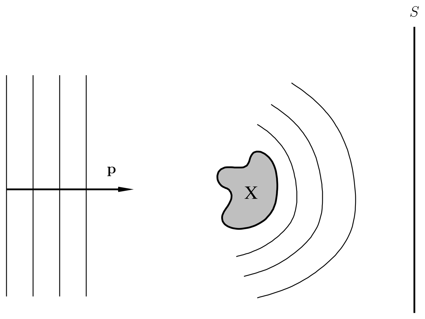
Figure 5:ure for problem \prbrpostulat-4. A scattering experiment.
Problem 4.
Measuring the Schr"odinger wave function is not like measuring a classical field, such as an electric field. Consider a scattering gedankenexperiment in which spinless particles of a given energy are directed at a target, as in the figure. We wish to measure the wave function downstream from the scatter. We assume the beam is described by a pure state, and that the incident wave is a plane wave (over a sufficiently large spatial region). The beam is low density, so the particles do not interact with one another. To measure over some volume of space, we just put a screen in a certain location, and gather enough statistics to get the probability density on this surface. We then move the surface and measure again.
Describe a modification to this gedankenexperiment by which the phase of the wave function can be measured on the screen, apart from the overall phase, which is nonphysical and can never be measured.