25. Fine Structure in Hydrogen and Alkali Atoms
Introduction
In these notes we consider the fine structure of hydrogen-like and alkali atoms, which concerns the effects of relativity and spin on the dynamics of the electron. Both these effects are of the same order of magnitude, and must be treated together in any realistic treatment of the atomic structure. In fact, spin itself may be thought of as a fundamentally relativistic phenomenon, although in low energy applications it is usually treated within a nominally nonrelativistic framework by the inclusion of extra terms in the Schr"odinger equation. This is the approach we shall take in these notes, where we treat the fine structure terms as perturbations imposed on the simple electrostatic model we have considered so far. The fine structure terms account for relativistic effects through order , and have the effect of enlarging the Hilbert space by the inclusion of the spin degrees of freedom, introducing new quantum numbers, and shifting and splitting the energy levels of the electrostatic model. The splitting in particular means that spectral lines that appear as singlets under low resolution become closely spaced multiplets under higher resolution (hence the term “fine structure”). The fine structure was known experimentally long before a proper theoretical understanding was achieved, and was an important driving force in theoretical developments at a certain stage in the history of atomic physics. In addition to its intrinsic interest and importance in atomic physics, the fine structure is interesting as a window on relativistic quantum mechanics.
The Hamiltonian
Our unperturbed system is a single-electron atom, hydrogen, hydrogen-like or alkali, in the electrostatic model. The unperturbed Hamiltonian is
where we ignore the small difference between the true electron mass and the reduced mass. As for the potential, for hydrogen-like atoms it is
whereas for alkalis it is the central force potential in the model discussed in Central Force Model of Alkali Atoms.
Now we add to the fine structure corrections, of which there are three: the relativistic kinetic energy correction, the Darwin term, and the spin-orbit term. We write the fine structure Hamiltonian as
which we will treat as a perturbation, to be added to the unperturbed Hamiltonian (1). We will discuss these terms one at a time, giving an idea of their physical significance.
The Relativistic Kinetic Energy Correction
Let us recall recall that the energy of a relativistic particle (rest mass plus kinetic energy) is
where we have expanded the square root in powers of the momentum, assuming . The first term is the rest mass, the second is the nonrelativistic kinetic energy, and the third is the correction,
The Spin-Orbit Correction
The spin-orbit term has the form,
where is the usual magnetic moment of the electron and is the magnetic field as seen in the electron rest frame (the prime refers to this frame). In the case of hydrogen, this magnetic field can be understood as due to the positive charge of the nucleus, which from the electron’s rest frame appears to be orbiting the electron, creating a current loop. In the case of the alkalis, the core electrons are also orbiting the valence electron, as seen in the rest frame of the valence electron, and contribute to the magnetic field in that frame.
Of course, the electron is accelerated, so its rest frame is not an inertial frame. This means that the simple picture we have described to explain the magnetic field in that frame does not give full accounting of the physics involved. In particular, it turns out that in relativity theory, an accelerated frame is associated with a rotation, called Thomas precession, which has an effect on the form of the spin-orbit interaction.
From another point of view, can be understood as the magnetic field that appears when we Lorentz transform the electrostatic field in the rest frame of the nucleus (what we may think of as the “lab” frame) to the frame of the electron. We will assume that there is no magnetic field in the “lab” frame. Actually, if the nucleus has a nonzero spin, then it produces a magnetic dipole field, which is responsible for the hyperfine interactions studied in 27. Hyperfine Structure in Atoms. But even when present, this dipole field is much smaller than the field responsible for the spin-orbit effects, so we shall ignore it here. Thus, using unprimed symbols , for the “lab” frame, we have
where we have used .
Now let be the velocity of the electron as seen in the “lab” frame, and the usual factor of time dilation in relativity,
where we have expanded in powers of . Then according to special relativity the electric and magnetic fields and seen in the frame moving with velocity with respect to the lab frame are given by
[See Jackson, Classical Electrodynamics, 3rd ed., Eq.~(11.149).] This is the general expression for the Lorentz transformation of electric and magnetic fields between two frames, but the formulas simplify quite a bit for our application, for which . Also, we are only interested in these formulas to lowest order in , which according to (8) means that we can approximate and drop the terms involving . This is because the spin-orbit term is already a small correction to the energy of the hydrogen atom, of order compared to the nonrelativistic energies. The result is
Now writing and using (7), we have
where . Then with
where we approximate , (6) becomes
The only remaining question is why there is a factor of in (6). We usually write the energy of a magnetic dipole in a magnetic field as . This factor is due to Thomas precession, a purely inertial effect of special relativity that causes accelerated frames to rotate relative to inertial frames. As we saw in Magnetic Resonance Experiments (see also Prob.~\jjcouple.1), inertial effects in a rotating frame can enhance or cancel out the effects of a magnetic field; in the present case, one half of the field is canceled.
Thomas precession is an interesting part of a study of special relativity, but it is probably overkill to go into it too deeply here, because the correct expression for the spin-orbit term, including the Thomas factor of , emerges automatically from the Dirac equation, which we will take up later in the course. For those who are curious, I have given a geometrical treatment of Thomas precession in my notes
{\tt http://
To summarize, the spin-orbit term is the magnetic energy of interaction of the spin with the magnetic field produced by the moving nucleus, corrected for Thomas precession.
The Darwin Term
The Darwin term is not as easy to interpret as the other two fine structure terms, but it can be described as a certain nonlocality in the interaction of the electron with the electrostatic field described by the potential . The following is a rough description of the physics lying behind the Darwin term.
If we confine an electron to a box of width , then by the uncertainty principle the momentum takes on values of the order of . If is small enough, we can make this momentum as large as we like, even relativistic values. Setting , a characteristic momentum at which relativistic effects are significant, and solving for , we obtain
where we now write for the length in question, which is called the Compton wave length. This is the distance scale below which the effects of relativistic quantum mechanics are important. This length can be defined for any particle, but in the case of the electron we have
where is the fine structure constant and is the Bohr radius. The electron Compton wave length is about times the size of the atom. Notice that this is still substantially larger than the size of the nucleus, .
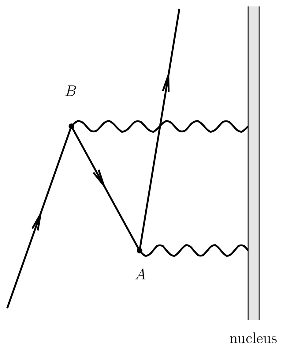
Figure 1:Feynman diagram for the creation of an electron-positron pair in the orbital motion of an electron in the hydrogen atom. The diagram is a space-time diagram with time increasing vertically, with the world-lines of the nucleus and electrons and a positron shown. Starting at the bottom, the electron in orbit around the nucleus enters at the left. Electron world-lines are indicated with an arrow pointing in the direction of increasing time. Later, at space-time point , a photon from the nucleus creates a positron electron pair, so that for a time there exist two electrons and one positron in the system. The positron world line is indicated with an arrow pointing backwards in time. At a later time, at space-time point , the incoming electron annihilates with the positron, producing a photon that is absorbed by the nucleus. After this, a single electron continues in its orbit, but, in a sense, it is not the same electron that entered at the bottom. The effect of diagrams like this is to smear the position of the atomic electron around in space over a distance comparable to the Compton wavelength.
If an electron is confined to a distance of order of the Compton wave length, then the corresponding momentum implied by the uncertainty principle implies an energy comparable to , the rest mass-energy of the electron. Then processes such as pair creation become possible, that is, the reaction,
where is the electron and is the positron. Such reactions do not literally occur inside an atom because there is not enough energy (a minimum of ) to create a positron-electron pair. But states containing two electrons and a positron do appear virtually, that is, for a period of time short enough that the violation of conservation of energy cannot be noticed (that is, times less than ). From another point of view, such virtual states appear in perturbation theory when one sums over “intermediate states,” which derive ultimately from a resolution of the identity. Such a sum can be seen in (8), the expression for the resolvent operator.
The positron-electron pair created according to (16) survives for a time of order , so, traveling at a velocity comparable to the speed of light, the particles cover a distance of order before disappearing again. The effect is to smear out the position of the atomic electron over a distance of order . The Feynman diagram for this process is shown in Figure 1.
To model this, let be a smearing function, normalized so that
The smearing function should be a positive function concentrated about with a width comparable to . Then the effective energy of interaction of the electron with a potential at position is not , but rather
Assuming that is slowly varying on the scale of , we can expand , obtaining
Because of the normalization (17) the first term is just , the usual expression for the potential energy of an electron at position . Assuming that is rotationally symmetric, that is, where , then the first correction term in (19) vanishes. As for the second term, let us assume a Gaussian model for the smearing function,
where the smearing length is the Compton wave length. Then we can do the integrals (see Appendix~\gaussint) for the second order term in (19),
Using this in (19) we obtain the energy correction,
The Darwin term is a term of exactly this form, but with a coefficient of instead of :
The Darwin term can be derived (with the correct coefficient) by performing a nonrelativistic expansion on the Dirac equation. See 49. The Foldy-Wouthuysen Transformation.
These pseudo-derivations of the fine structure terms are not completely satisfactory, but for now we will just accept them and use them for practice in perturbation theory.
Specializing to Hydrogen-like Atoms
To simplify the notation we switch now to atomic units, which were explained in Atomic Units. See Table 1. Notice that in atomic units the fine structure constant becomes
Since the fine structure constant is dimensionless, it has the same value in all systems of units. Thus, the speed of light in atomic units is , and the velocity of the electron in the ground state of hydrogen is given by .
Translating the three fine structure terms, (5), (13) and (23) to atomic units, we have
Notice the common factor of in front of all three terms.
If we evaluate the spin-orbit and Darwin terms explicitly for hydrogen-like atoms, for which , , and , then we obtain
The quantity occurring in the Darwin term is the charge density of the nucleus, treated as a point charge. We will henceforth in these notes specialize to the case of hydrogen-like atoms, returning to the case of alkalis briefly at the end.
All three fine structure terms (25) are multiplied by , which is about . As we shall see, these terms all give corrections to the energies of the electrostatic model that are of relative order , which is correspondingly small if is not too large. This is what we should expect for relativistic corrections, since the velocity of the electron in the ground state of a hydrogen-like atom is of the order of , and we expect relativistic corrections to the energy to go like . Toward the end of the periodic table, however, is no longer so small ( for uranium), and it ceases to be a good approximation to treat relativistic effects as corrections superimposed on a nonrelativistic model. In such heavy atoms the fine structure corrections are becoming comparable to the separation between the levels of the electrostatic model, and it is no longer useful to treat them as perturbations imposed on that model. Instead, it is more useful to start with a proper relativistic treatment of the electron, which is the Dirac equation.
The Unperturbed System
We now consider applying as a perturbation to . As usual in perturbation theory, we must first understand the unperturbed system. The unperturbed energy levels are
If we ignore spin, the unperturbed eigenstates are , that is, they are central force wave functions, and they are -fold degenerate. However the spin-orbit term (27) explicitly involves the spin, so we must enlarge our Hilbert space to include the spin degrees of freedom. We write
[see (11)] for the entire Hilbert space of the electron, where a convenient basis in is the set of unperturbed central force eigenfunctions , and where we use the usual basis in . We put subscripts on the magnetic quantum numbers and to indicate what kind of angular momentum they represent (orbital and spin, respectively). The products of these basis states form a basis in ,
what we shall call the uncoupled basis. This basis is an eigenbasis of the complete set of commuting observables corresponding to quantum numbers . The quantum number corresponding to the operator is suppressed, because it is constant [, ]. Since the unperturbed Hamiltonian (1) is a purely orbital operator, including the spin degrees of freedom does not change the unperturbed energy eigenvalues (30), but it does double the degeneracies (to ), since there are two spin states (“up” or “down”) for each orbital eigenfunction.
Choosing a Good Basis in Degenerate Perturbation Theory
Since the unperturbed energy levels are degenerate, we must think in terms of degenerate perturbation theory, in which the shifts in the energy levels are the eigenvalues of the matrix of the perturbing Hamiltonian in the eigenspaces of the unperturbed system. In the present case, the unperturbed levels are -fold degenerate, so we will have a matrix. This matrix will be easier to diagonalize in some bases than others.
The following describes a simple procedure for choosing a good basis. To take a specific example, let be some perturbing Hamiltonian, perhaps one of the fine structure terms. If we use the uncoupled basis (32), then the matrix elements needed in perturbation theory are
Notice the distribution of primes: the index is the same on both sides of the matrix element because it labels an unperturbed eigenspace, while the indices , and are allowed to be different, since these label the basis states inside the unperturbed eigenspace. Suppose now that . Then we have
so either or else the matrix element (33) vanishes. This example illustrates a general principle, which is that if an operator commutes with an observable belonging to a complete set of commuting observables, then the operator has diagonal matrix elements with respect to the quantum number of the observable in the eigenbasis of the complete set. This rule can often be used in cases where the Wigner-Eckart theorem does not apply. Its importance for degenerate perturbation theory is that in setting up the matrix elements of the perturbing Hamiltonian, we should use an eigenbasis of a complete set of commuting observables in which as many as possible of the observables commute with the perturbing Hamiltonian. If we are lucky or clever, the perturbing Hamiltonian will commute with all members of some complete set of commuting observables, and then its matrix elements will be entirely diagonal. In this case, the eigenvalues are the diagonal elements, and degenerate perturbation theory will have been effectively reduced to nondegenerate perturbation theory (that is, one obtains energy shifts just by computing expectation values, and one will not have to diagonalize any matrices).
A Good Basis for the Fine Structure Perturbations
Therefore in analyzing the fine structure perturbation, we should look for observables that commute with . The results are summarized in Table 1. We start with . This is a purely orbital operator, and is furthermore a scalar. Therefore it commutes with , the generator of orbital rotations. Also, since it is purely an orbital operator, it commutes with , which implies that it also commutes with . Furthermore, since it commutes with , and , it commutes with any functions of them as well, including , and . The term is similar; it is also a purely orbital operator, which is a scalar. (The -function can be thought of as the limit of a highly concentrated, rotationally symmetric function centered on , which therefore commutes with .) Therefore also commutes with , , , , and . However, the term does not commute with either or , since either purely spatial or spin rotations would rotate one half or the other of the dot product , and would not leave the dot product invariant. However, does commute with , which generates overall rotations of the system and which rotates both and simultaneously. It also commutes with and , because of the commutators, and , and with , because it commutes with .
Table 1:The table indicates whether the given fine structure term commutes with the given angular momentum operator (, ).
FS Term | ||||||
|---|---|---|---|---|---|---|
Y | Y | Y | Y | Y | Y | |
Y | Y | Y | Y | Y | Y | |
N | Y | N | Y | Y | Y |
We see that and are diagonal in the uncoupled basis (32), but that is not. However, all three operators are diagonal in the eigenbasis of the operators . This suggests that we use the coupled basis for the perturbation treatment, that is, the basis in which we have combined angular momenta according to or , as in 18. Coupling of Ket Spaces and the Addition of Angular Momenta. Following (50), we define the coupled basis in terms of the uncoupled basis by
where the matrix element is a Clebsch-Gordan coefficient, and where we have suppressed the constant quantum number in various places.
Since all three fine structure terms are diagonal in the coupled basis, we only need to compute their diagonal matrix elements and add them up to get the fine structure energy shifts. This is the optimal situation in degenerate perturbation theory; there are no matrices to diagonalize.
Some books, for example, Bransden and Joachain, diagonalize and in the uncoupled basis, and in the coupled basis, and then add the eigenvalues. This gives the correct answer for this problem but such a procedure cannot be recommended in general since the eigenvalues of a sum of matrices is not equal in general to the sum of the eigenvalues.
The Energy Shift for 
We begin with in (25), for which the desired matrix element is
where we have expressed the coupled basis vectors in terms of the uncoupled basis. We do this because , being a purely orbital operator, is easier to evaluate in the uncoupled basis. Since does not involve the spin, the middle matrix element in (37) becomes
where the last matrix element is purely orbital. In fact, it is the matrix element of a scalar operator with respect to a standard angular momentum basis (under orbital rotations alone), so by (54), the Wigner-Eckart theorem for scalar operators, it is equal to times a quantity that is independent of magnetic quantum numbers. That quantity can be regarded as a reduced matrix element, or it can be taken as the given matrix element with some convenient set of magnetic quantum numbers inserted, since the answer doesn’t depend on them anyway. The value zero is convenient, so we have
When we put (38) and (39) back into (37) and use the orthogonality of the Clebsch-Gordan coefficients [see (54)], we find simply
The energy shifts due to , which nominally depend on , , and , actually depend only on and . We might have guessed this, since is diagonal in both the coupled and uncoupled basis (and the answer could not depend on in any case, since is a scalar operator).
We can now evaluate the final, purely orbital matrix element. We do this by writing
where is the kinetic energy. Then we have
The final expression involves expectation values of powers of ; the angular integrations are trivial because of the orthonormality of the 's, and the remaining integration is over the radial variable . The needed expectation values for hydrogen-like atoms are
(see Prob. Paragraph) which after some algebra give the final answer in the form,
Here we have factored out the unperturbed energy to show that the energy corrections are of order compared to the energy scale of the unperturbed system.
Energy Shift for the Darwin Term
The analysis of the Darwin term of (28) is similar. Since it is also a purely spatial scalar operator, its matrix element reduces as in (40),
where the -function has allowed us to do the integral. Here
is the normalized energy eigenfunction. But because of the boundary conditions for small , the answer will be nonzero only for (-waves). Using and the property of the hydrogen-like radial wave functions,
which can be derived from (21) and (28), we can write the final answer in the form,
The Spin-Orbit Energy Shift
Finally, we consider the spin-orbit term, of (29). Because of the identity,
its matrix elements can be written,
The remaining matrix element is again of a purely spatial scalar operator, which can be reduced to a purely spatial matrix element as in (40). The result becomes the expectation value of , which in a hydrogen-like atom is given by
This expectation value diverges for . But in that case, the operator is the zero operator, so we seem to have the form for the energy correction. The proper way to handle this is to smooth out the Coulomb singularity at , whereupon the expectation value of does not diverge, and the answer is seen to vanish for . Altogether, we can summarize the answer for by
The Total Fine Structure Energy Shift
All three fine structure corrections, (46), (50), and (54), are of order times the unperturbed energy levels, as predicted. When we add them up to get the total energy shift due to the fine structure, the result simplifies after some algebra, and we find
The most remarkable thing about this answer is that it is independent of the orbital angular momentum quantum number , although each of the individual terms does depend on . However, the total energy shift does depend on in addition to the principal quantum number , so when we take into account the fine structure corrections, the energy levels of hydrogen-like atoms have the form . Of course the levels do not depend on because the Hamiltonian is a scalar operator. Factoring out the unperturbed energy levels, we can write the total energy of a hydrogen-like atom in the form,
The ellipsis indicates higher order terms that we have not calculated, but it is easy to believe that they turn into a power series in the quantity .
Comparison With the Dirac Equation
The Dirac equation for a hydrogen-like atom can be solved exactly. This does not mean that the answers agree exactly with the physics, because the Dirac equation, although fully relativistic, omits some important physics that we will consider later. Nevertheless, it is interesting to compare the results of the Dirac equation with the results of our perturbation calculation above. The Dirac energy levels are
where we revert to Gaussian units. See Recursion Relations and Energy Levels for details. When this expression is expanded in powers of , we obtain,
The first term in this expansion is the rest mass-energy, , the next contains the nonrelativistic Bohr energy levels , and the third contains the fine structure corrections (55). Each term is of order times the previous term.
There is no point in expanding the solution of the Dirac equation beyond the fine structure term, because there are other physical effects that are not incorporated into the Dirac equation that are larger than the next term after the fine structure term. Most important of these are the hyperfine effects, discussed in a subsequent set of notes, and the Lamb shift, discussed in The Lamb Shift.
Hydrogen-Like Energy Levels in the Fine Structure Model
Let us call the model of a hydrogen-like atom that includes the fine-structure perturbations the fine structure model. It is a refinement on the nonrelativistic, spinless, electrostatic model we have considered previously. We now examine some features of the energy levels in the fine structure model of a hydrogen-like atom.
The energy shifts (55) are negative for all values of and , so fine structure effects depress all energy levels. However, smaller values of are more strongly depressed, so the total energy (unperturbed plus fine structure) is an increasing function of . Since the unperturbed levels did not depend on , fine structure effects have partially resolved the degeneracy in the unperturbed levels, which now have the form (instead of just ). The fact that the levels still do not depend on means that the hydrogen atom, even including relativistic corrections, still has some extra symmetry that goes beyond rotational invariance (in particular, there is still a degeneracy between states of opposite parity).
In first courses on quantum mechanics the spin-orbit term is frequently the only term considered in treatments of the fine structure. It is true that this term alone is responsible for the -dependence of the perturbed energy levels and their splitting, but unless the relativistic kinetic energy and Darwin terms are also included, one misses the fact that the total fine structure energy shifts are independent of . It is clear from the formula (57) that this -degeneracy persists to all orders in the expansion of the Dirac equation in powers of .
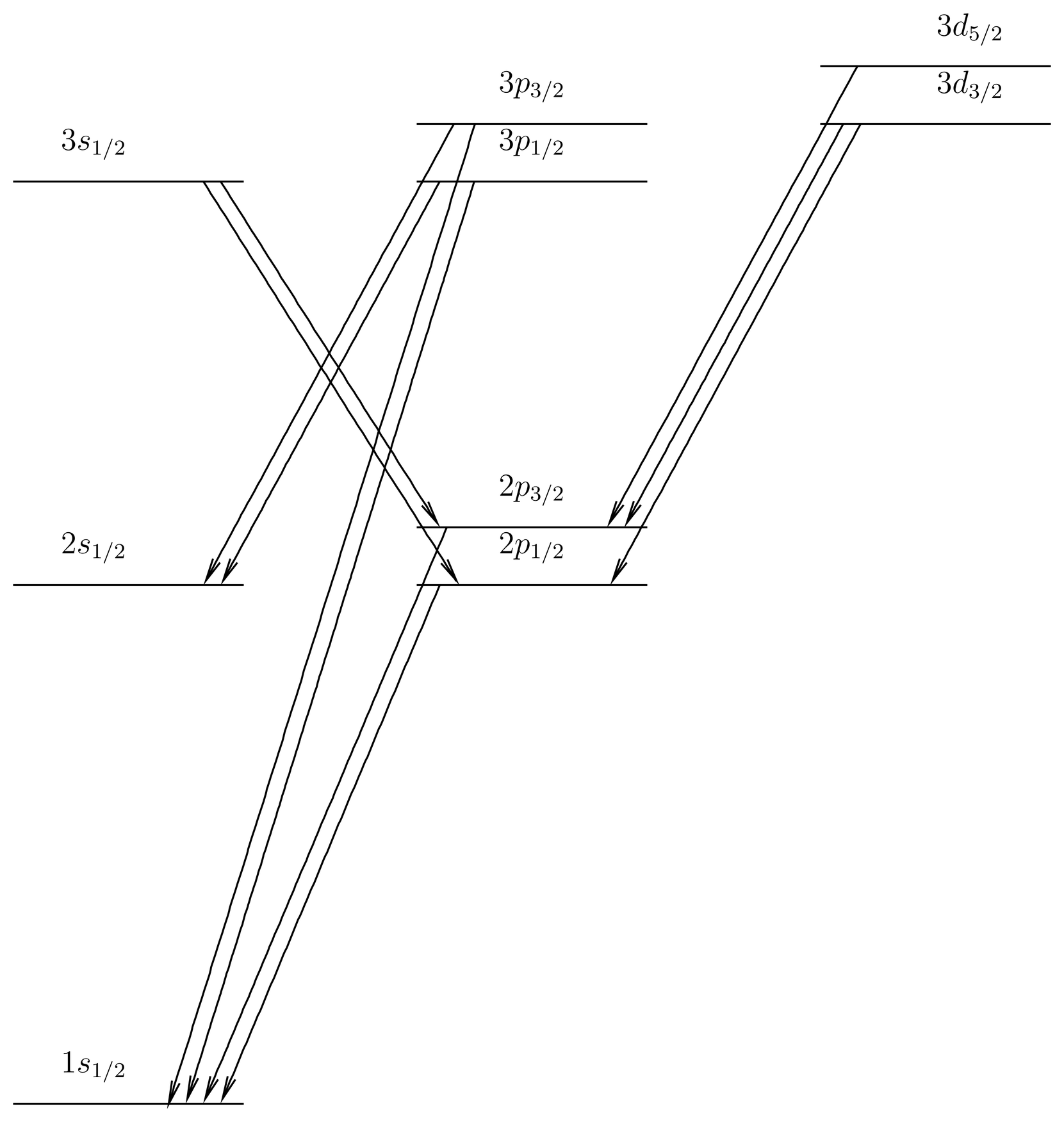
Figure 2:Energy level diagram for hydrogen or hydrogen-like atoms, including fine structure, with allowed electric dipole transitions indicated (Grotrian diagram). Not shown are transitions only involving small energy differences, such as . Diagram is schematic and not to scale; in particular, the fine structure splittings are of order times the separation between the levels of different .
The standard spectroscopic notation for the states of hydrogen-like or alkali atoms is , where is represented by one of the standard symbols, , , , , etc. For example, the ground state of hydrogen is the level. The low lying levels in a hydrogen-like atom are indicated schematically in Figure 2.
Electric Dipole Transitions in Hydrogen-Like Atoms
Figure 2 also indicates the most important electric dipole transitions in a hydrogen-like atom. Allowed electric dipole transitions, , are those for which the matrix element
is nonzero, where is the component of the position operator with respect to the spherical basis (37). The operator is a irreducible tensor operator, both under purely spatial rotations, generated by , and under rotations of the whole system, generated by . Therefore the Wigner-Eckart theorem can be applied twice. When it is applied to purely spatial rotations and combined with parity, it gives the selection rule ( would be allowed by the Wigner-Eckart theorem, but is excluded by parity). When the Wigner-Eckart theorem is applied to total rotations, it gives the selection rules and . There is nothing to exclude transitions with , and, in fact, such transitions occur. The selection rule involving magnetic quantum numbers gives information about the polarization of the photon emitted on transitions from some initial to some final magnetic substate.
Concerning parity, note that it is a purely orbital operator that has no effect on spin. Thus its action on states of the uncoupled basis is
From this and from (35), the action of parity on the states of the coupled basis is
The Lamb Shift
The Lamb shift is a shift in the energy levels of the Dirac picture that is due to the interaction of the electron with the vacuum fluctuations of the quantized electromagnetic field. It has small effects on all the energy levels, and its most notable feature is that the effect is different on levels with the same values of and but different values of . Thus, including the Lamb shift, the energy levels in hydrogen have the form , and the only degeneracy is that due to rotational invariance. All extra or “accidental” degeneracy is removed.
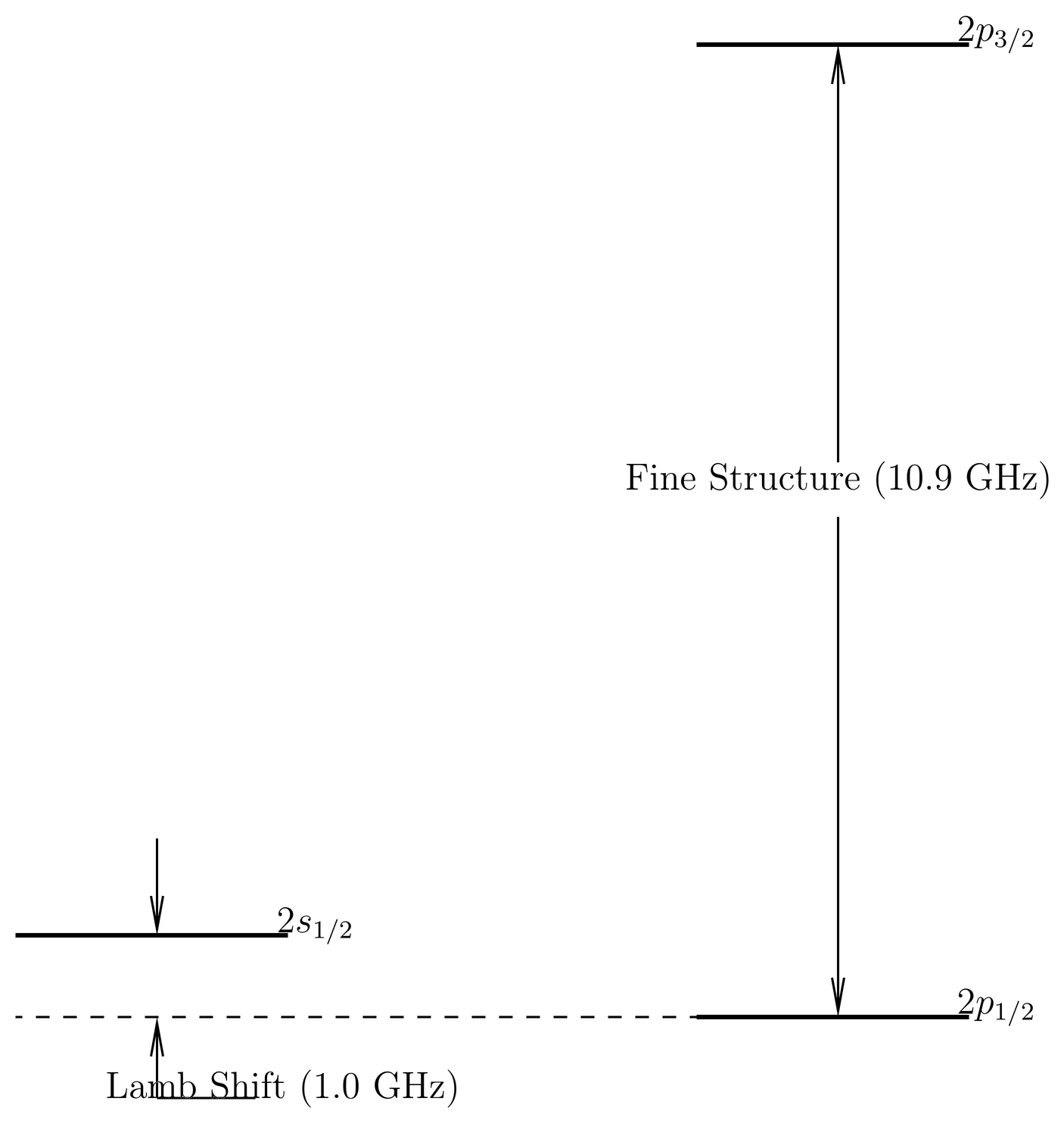
Figure 3:An expanded view of the levels in hydrogen, including the Lamb shift. The splitting due to the Lamb shift is notable because it introduces an -dependence into the energies. Its magnitude is about 10 times smaller than the fine structure splitting (on the levels).
The most important manifestation of the Lamb shift is in the levels of hydrogen. See Figure 3. Here the Lamb shift causes the level to be raised about 1.0~GHz relative to the level. This energy difference can be measured with high accuracy with radio frequency techniques. The detection and theoretical calculation of the Lamb shift was an important milestone in the history of quantum electrodynamics, because it was one of the first successful application of renormalization theory. We will consider the Lamb shift in more detail in later in the course.
Fine Structure in Alkali Atoms
Most of the analysis presented above for hydrogen-like atoms goes through for the alkali atoms, with replaced by the appropriate screened Coulomb potential. The unperturbed (nonrelativistic) energy levels of the alkalis have the form , and are already strongly split by the values because of the non-Coulomb nature of the central force. See Fig.~\figr\hydrogen.3 for the case of sodium. The three fine structure terms present in hydrogen are also present in the alkalis, but the relativistic kinetic energy and Darwin terms are not very interesting, because they cause only small shifts in the energy levels of , without splitting them. That is, the energy shifts produced by these terms have the form , and the energies already depend on and . These terms are more interesting in hydrogen, because of the degeneracy among the different values. However, the spin-orbit term does split the alkali levels according to their values, much as in hydrogen, and produces overall energy levels of the form . The analysis of the spin-orbit splitting in the alkalis proceeds much as with hydrogen in The Spin-Orbit Energy Shift, yielding
The expectation value is with respect to the wave function ; it must be done numerically since both and are only known numerically. But the formula (62) does give the correct dependence on the quantum number .
The levels of sodium displayed in Fig.~\figr\hydrogen.3 do not show the fine structure splitting, because it is too small on the scale of that diagram. But, for example, if the level is examined closely, it will be found to be split into a level and a level, with the level lying 0.00213~eV above the level. This causes the transition (the yellow sodium -line) to be a close doublet. The selection rules in the alkali atoms depend only on the angular momentum quantum numbers, and are the same as in hydrogen.
Problems
Problem 1.
If a hydrogen atom finds itself in the state (either or ) it will emit a photon and decay into the ground state in about 10-9 seconds. If it finds itself in the state, however, it will remain there much longer.
(a) Explain why the transition } is not allowed as an electric dipole transition. However, due to the Lamb shift, the state is 1.0 GHz below the state, and the electric dipole transition is allowed. If the atom makes this transition, it will almost immediately drop into the ground state, so the rate of the transition is effectively the decay rate via this mechanism.
(b) It can be shown that rate for an electric dipole transition (in ) is
where and are states of a single electron atom, and where is the frequency of the emitted photon. Also, you may note that
where is the component of the position vector with respect to the spherical basis, as in The Nucleus and the M"ossbauer Effect.
Suppose the initial state is . Find the transition rate to any state, as an electric dipole transition. You have to sum the rates to any final state that is accessible from the initial state.
I suggest you first express the matrix elements of with respect to the hydrogen atom states in the fine structure model, , in terms of the matrix elements of with respect to the states of the electrostatic model, . Then evaluate the latter any way you can, for example, by the method described in The Nucleus and the M"ossbauer Effect.
Problem 2.
When a spectral line of hydrogen associated with a transition between two states of the electrostatic model, for example, , is examined under high resolution, it appears as a multiplet, due to the fine structure. How many lines will be seen associated with ? The transition has the same energy as , in the electrostatic model. How many lines will be seen when the fine structure is taken into account?