06. Topics in One-Dimensional Wave Mechanics
Introduction
In these notes we consider some topics that arise when solving the time-independent Schr"odinger equation for potential motion in one dimension. I have borrowed most of this material from the lecture notes of Professor Eugene Commins. The Schr"odinger equation is
Degeneracies in One Dimension
Let and be two solutions of (1) corresponding to the same energy , so that
We multiply the first equation by and the second by and subtract, to get
where is the Wronskian of the two solutions,
Thus, is a constant (independent of ).
Now suppose (usually due to boundary conditions) that both and vanish at some point . We include the possibilities , , or both. Then everywhere, so
which implies
where is a constant.
We see that if both and vanish anywhere on the -axis, including , then they are proportional to one another. There is no degeneracy.
Bound state eigenfunctions die off exponentially outside the classically allowed region, so these go to zero at both infinities and must be nondegenerate. In a potential such as that sketched in Fig.~\figr\hilbert.4, the positive energy eigenstates are not bound, but they do die off exponentially at one of the infinities, and so are nondegenerate. In the case of a potential that approaches zero at both infinities, positive energy eigenfunctions do not approach zero at either infinity, so the theorem just proved does not forbid degeneracies. In fact, such eigenfunctions are two-fold degenerate, as can be seen from the case of the free particle, where are both eigenfunctions of energy .
The Reality of Energy Eigenfunctions
Since the Schr"odinger equation (1) is real, if is a solution of energy , then so is . But if the energy is nondegenerate, then and must be proportional,
for some constant . By squaring both sides we have
which shows that must be a phase factor, . Therefore
Now defining
we see that is real. We conclude that any nondegenerate energy eigenfunction in one dimension is proportional to a real eigenfunction. In other words, by a phase convention, the nondegenerate eigenfunctions can be chosen to be real.
In the case of degenerate eigenfunctions, it can be shown that one can always choose linear combinations that are real. For example, in the case of the free particle we have degenerate, complex eigenfunctions . But by forming linear combinations, we can create the real eigenfunctions and .
These results are a special case of time-reversal invariance, which is studied in a more general and systematic way later in the course. See 22. Time Reversal.
Interleaving of the Nodes
The zeros of an energy eigenfunction are called its nodes. Suppose the potential supports some bound states, with energies . We know these energies must be nondegenerate. Then it can be shown that the -th excited bound state with energy has precisely nodes. Moreover, the nodes interleave one another, that is, the nodes of lie between the nodes of . This can be seen in some examples such as the harmonic oscillator. See Figs.~Figure 1 and Figure 2. The proof of these facts may be found in Morse and Feshbach.
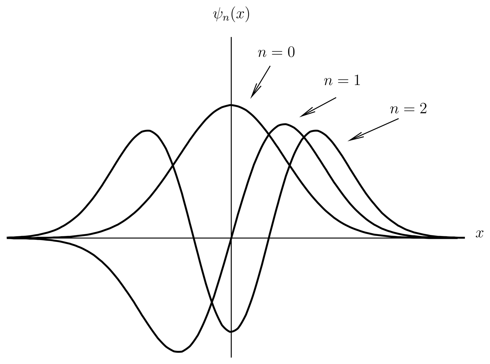
Figure 1:Eigenfunction has nodes. Harmonic oscillator eigenfunctions are illustrated for .
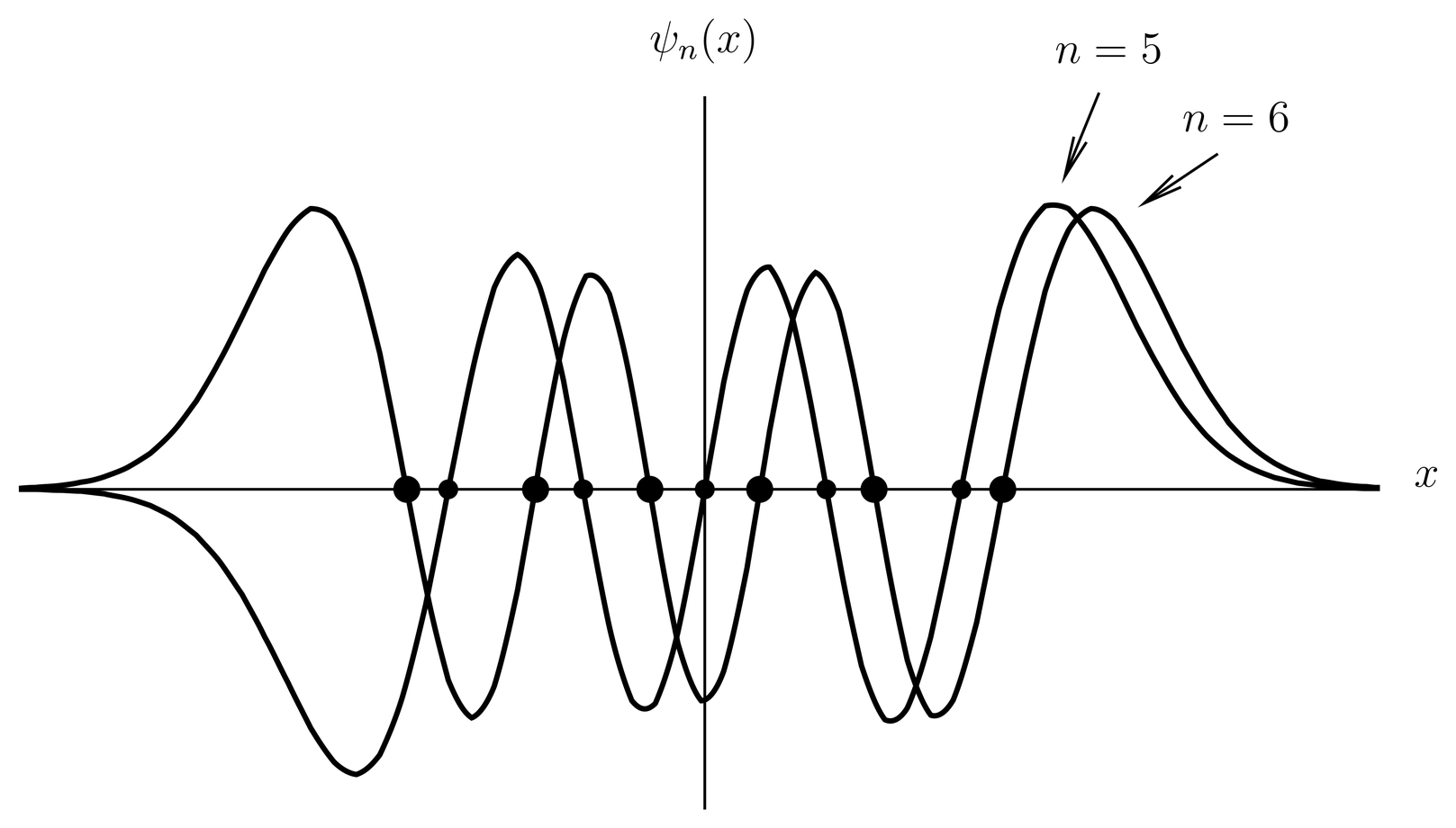
Figure 2:The nodes of successive eigenfunctions interleave, here illustrated for . The small dots are the nodes for , the large ones for .
Here is an application. Consider the double well oscillator, whose potential is sketched in Figure 3. If the barrier in the middle is high, then tunnelling is small and the ground state wave functions in the left and right wells do not communicate with each other very much. Thus, both and are nearly ground states for the whole potential, and there is a near degeneracy.
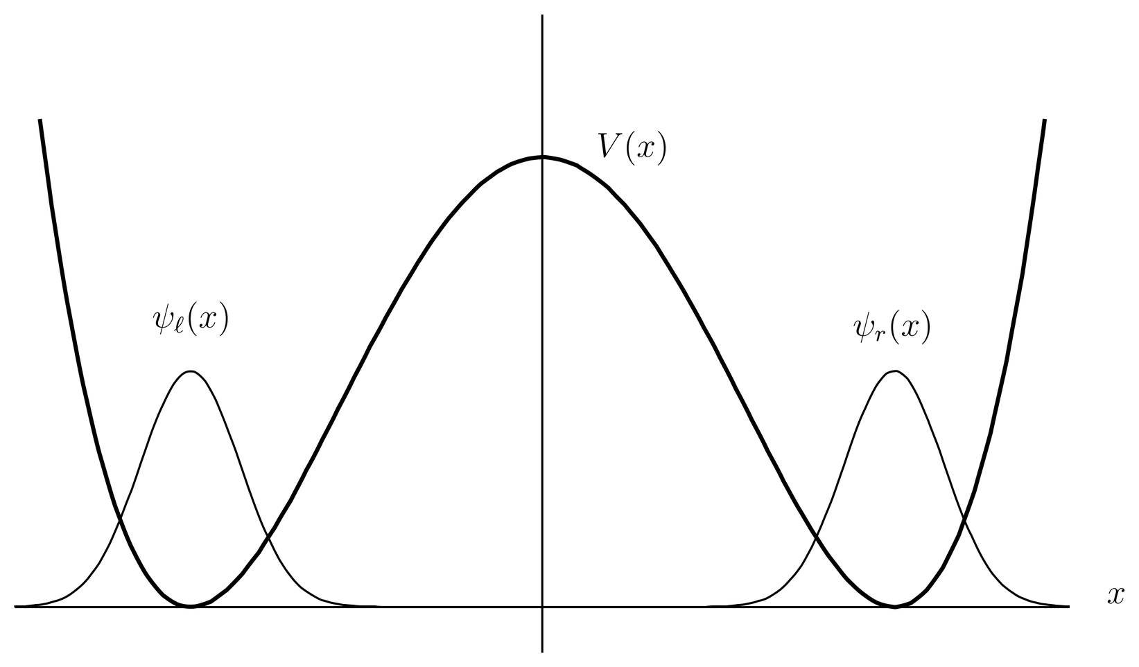
Figure 3:A double well potential (heavy line). Also shown are the approximate ground state wave functions in the left and right wells.
As shown in Degeneracies in One Dimension, however, there cannot be an exact degeneracy. Now since the Hamiltonian commutes with parity, by Theorem Theorem the eigenstates of , which are nondegenerate, must also be eigenstates of parity. Since and are not eigenstates of parity, to get the energy eigenstates we must form symmetric and antisymmetric linear combinations,
which are illustrated in Figs.~Figure 4 and Figure 5. These are eigenstates of parity.
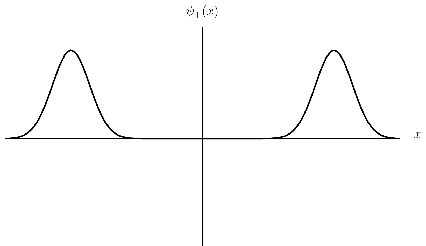
Figure 4:Even eigenfunction in double well potential.
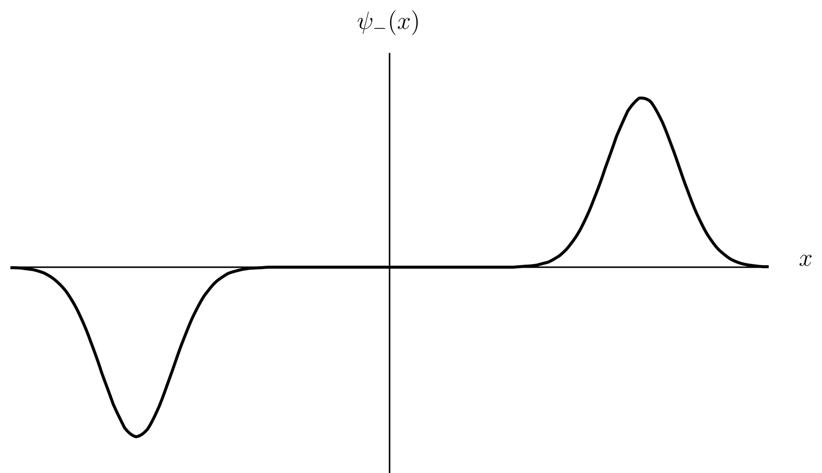
Figure 5:Odd eigenfunction in double well potential.
But which one of them is the ground state, and which the excited state? According to the rules we have presented, the symmetric state in Figure 4 has no node, and must be the ground state, while the antisymmetric state in Figure 5 has one node and must be the first excited state.
Problems
Problem 1.
A -function potential is often a useful model, especially in one-dimensional problems. The potential
can be seen as the limit of a square well potential,
as . The parameter has dimensions of energy times distance. The potential shown is a -function well potential (for ), but by changing the sign of we get a -function barrier.
Show that the -function well supports precisely one bound state. Find the energy and the wave function.
Hint: This can be done by taking the limit of a square well solution, but the following is an easier method.
Normally we require the wave function and its first derivative to be continuous in in a one-dimensional solution of the Schr"odinger equation. If the first derivative had a discontinuity, it would mean that the second derivative, which appears in the kinetic energy term, would have a -function at the location of the discontinuity of the first derivative. That -function can only be balanced out in the Schr"odinger equation if the potential has a -function. However, in the present situation, that is precisely what we have.
So solve the Schr"odinger equation in the region and , where , and then find the discontinuity in across by integrating over a small interval .