50. Solutions of the Dirac Equation and Their Properties
Introduction
In 46. Introduction to the Dirac Equation{} we introduced the Dirac equation in much the same manner as Dirac himself did, with the motivation of curing the problems of the Klein-Gordon equation. We saw that the Dirac equation, unlike the Klein-Gordon equation, admits a conserved 4-current with a nonnegative definite time component, so that it can be interpreted as a probability 4-current. On the other hand, the Klein-Gordon equation has one problem that is shared with the Dirac equation, the existence of negative energy solutions, for which we have no interpretation as yet. We might suppose that the negative energy solutions could simply be declared to be nonphysical, but this turns out to be impossible, as we will see. In addition, the velocity operator in the Dirac theory is strange, being a purely spin operator when we might have expected something purely spatial on the nonrelativistic analogy. The same velocity operator appears in the spatial part of the probability current. It is however encouraging that the Dirac equation automatically produces the correct interaction of the spin with a magnetic field, with the (almost exactly) correct -factor for an electron. To summarize, as a candidate relativistic wave equation for the electron, the Dirac equation presents some remarkable successes, some strange features, and some others with no obvious physical interpretation.
The purpose of these notes is to explore some solutions of the Dirac equation and their properties, in order to accumulate some results that will be useful for later work, to reveal some further successes of the Dirac equation, and to explore some of the puzzling aspects of the theory in order to understand them better and to lay the foundation for their ultimate resolution.
We begin by exploring the properties of free particle solutions of the Dirac equation, including the negative energy solutions. The free particle solutions form a basis of orthonormal eigenfunctions that will be useful for later work, especially when we turn to the second quantization of the Dirac field. We do not manage at this time to obtain a physical interpretation of the negative energy free particle solutions, but we learn some things about them, such as their energy spectrum and the fact that, in a certain sense, they have negative momentum and spin as well as negative energy. We then turn to the Gordon decomposition of the current, which gives some understanding as to why the velocity appears as a spin operator in the Dirac theory. Then we present a discussion of the Zitterbewegung, a kind of jittering motion that the Dirac electron undergoes on a rapid time scale, even in the case of a free particle. The Zitterbewegung is related to the Darwin term in atomic physics (see 25. Fine Structure in Hydrogen and Alkali Atoms). Finally, we discuss central force problems in general and then the exact solution of the hydrogen atom for the Dirac equation. This gives us not only all the fine structure corrections we saw in 25. Fine Structure in Hydrogen and Alkali Atoms{} but also negative energy solutions. For these, however, as in the case of the free particle, we have no interpretation as yet.
The net effect of this set of notes will be to give us experience with some exact solutions of the Dirac equation (the free particle and the hydrogen atom), some understanding of some of the strange features (the velocity operator), some new strange features (the Zitterbewegung), and yet still no physical interpretation of the negative energy solutions (that will come later).
In the following treatment of free particle solutions it will be important to distinguish the momentum operator (3-vector or 4-vector) from the corresponding vectors of -numbers. Therefore we will put an “op” subscript on the momentum when an operator is intended, such as or , and omit the “op” subscript when a -number is intended. For other operators the distinction will not be necessary so we will omit the “op” subscripts. We will use hats on unit vectors, as usual.
Free Particle Solutions of the Pauli Equation
The Pauli Hamiltonian for a free particle of spin is and the wave function is a 2-component spinor. A complete set of commuting observables that also commute with the Hamiltonian is . The eigenfunctions of that are also eigenfunctions of these observables are
where is the momentum eigenvalue, where the first solution is an eigenfunction of with eigenvalue and the second with eigenvalue . We have included the time dependence in these solutions, where .
Dirac Free Particle Solutions and Spin
The Dirac Hamiltonian for a free particle is
In comparison to the Pauli theory, we might expect to find eigenfunctions of that are also eigenfunctions of and , the latter being the Dirac generalization of the Pauli operator . This does not work, however, for although and commute with each other (one is purely spatial and the other purely spin), and although commutes with , does not commute with . This is because generates spin rotations, which rotate the vector but not the spatial vector , so the dot product is not invariant. On the other hand, orbital angular momentum generates spatial rotations that rotate but not , so again is not invariant. Obviously if we want to find an angular momentum operator that does commute with , it is , the total angular momentum (orbital plus spin) of the Dirac particle. See Angular Momentum of the Dirac Particle.
Although orbital and spin angular momentum are defined for the Dirac particle, they are not separately conserved, even for a free particle. This is a reflection of the more intimate coupling of orbital and spin degrees of freedom in the relativistic theory, as compared to nonrelativistic quantum mechanics. Recall that for the photon, orbital and spin angular momentum are separately not even defined, although is.
On account of these considerations, we can expect spin to play a more complicated role in the theory of free particle solutions of the Dirac equation than it does in the Pauli theory.
Free Particle Solutions of the Dirac Equation at Rest
There are four linearly independent solutions of the time-dependent Dirac equation for a free particle at rest. These are given in (31), reproduced here:
The first two of these have energy , and the last two have energy , as we find by applying either or . We have as yet no physical interpretation for the solutions of negative energy, but they will turn out to be important so we must keep them and investigate their properties.
The solutions at rest, (3), are eigenstates of , that is, the spin is polarized in the direction in the rest frame. In following work we will want to be more general, and to allow the spin to be polarized in an arbitrary direction in the rest frame. Let be a unit vector in the rest frame of the particle. If are the angles of in spherical coordinates, then we define the 2-component (Pauli) spinor as the spinor “pointing in” the direction , as explained in A Spin “Pointing In” a Given Direction. According to (67), this spinor is
to within an overall phase which will not be important to us. In this notation the eigenspinors of are ,
the second of which follows by making the replacement in the first. For a fixed value of , the spinors form an orthonormal basis in the space of 2-component spinors.
Now we define two types of 4-component spinors, here broken into their upper and lower 2-component spinors,
where the 0 subscript on and means, “at rest.” The odd thing about these definitions is that we have used in the definition of , that is, with a minus sign on the direction of spin. The reason for this choice will be explained momentarily. These spinors are eigenspinors of the Dirac matrix , where
(this is (61). That is,
Then the most general free-particle solutions of the Dirac equation when the particle is at rest can be written
of which the first has energy and the second . These are the positive- and negative-energy solutions, respectively. If is chosen to run over two oppositely oriented unit vectors in the rest frame, then the solutions (9) constitute a complete set of free particle solutions at rest, with definite spins in the rest frame.
Boosting the Solutions at Rest
To create free particle solutions in some state of motion we apply a boost to the free particle at rest. We first consider this problem from a classical standpoint. Let be the desired 3-momentum of our particle, and the boost that will take the particle at rest into one with momentum . The 4-momentum of the particle at rest is
where again the 0-subscript means “at rest” and the 4-vector is given in -notation. The 4-momentum of the particle after the boost is
where
This is of course the standard definition of the energy of a free particle in relativity theory, but in the following it will be important to remember that the symbol stands for the positive square root in (12), even when we are talking about negative energy solutions. Also, in the following both the energy and the 4-momentum will be understood to be functions of the 3-momentum , which by itself characterizes the state of motion of the particle after the boost.
We can put the boost into axis-rapidity form, as in Pure Boosts. The boost must be in the direction of the momentum so the boost axis is
where is a unit vector, and its rapidity is given implicitly as a function of by
where is the velocity of the particle after the boost. With this axis and rapidity, we have . The action of a boost in axis-rapidity notation on an arbitrary 4-vector is given explicitly by (34). Applying that equation, we can check that
We shall sometimes write this as , using simply and for the 4-momenta with components and .
We turn now to the quantum side of the boost, that is, boosting the free particle solutions at rest, (9), of the Dirac equation. In this process it will be convenient to use covariant notation insofar as possible. As for the exponents in (9), notice that
in the notation of (104) for the Minkowski scalar product of two 4-vectors. Therefore we can write the positive and negative energy solutions for a free particle at rest as
Under the Lorentz transformation , a Dirac 4-component wave function is mapped into , as explained in Transformation of the Dirac Wave Function, where we define
Under this mapping, the exponents in (17) transform according to
where we use the identity (105). This calculation is essentially the same as that presented in The Space-Time Part of the Transformation. As for the matrix , the -matrix in axis-rapidity notation is given by (75). Here we express the hyperbolic functions of half-angles in terms of the energy and momentum of the particle after the boost, as follows:
Substituting these into (75), we obtain the explicit form of the -matrix,
Under the Lorentz transformation acts on the spinors , , giving us boosted spinors that we will write as
without the 0-subscript. The boosted positive and negative energy solutions are now
If we apply or to these to obtain their energies, we find that the positive energy solutions have energy , given in terms of the momentum which parameterizes the boost by (12), while the negative energy solutions have energy . We see that when we boost a negative energy solution at rest, we obtain a solution whose energy is even more negative. Thus, the energy spectrum of the free particle Dirac Hamiltonian consists of a positive energy part ranging from to , and a negative energy part ranging from to , as illustrated in Figure 1. There is an energy gap between and .

Figure 1:The energy spectrum of the free particle Dirac Hamiltonian consists of all positive energies and all negative energies . There is an energy gap between and .
The free particle solutions (23) are not only eigenfunctions of energy, they are also eigenfunctions of momentum. If we apply the operator to these solutions, we find that positive energy solutions are eigenfunctions of momentum with eigenvalue , while the negative energy solutions are eigenfunctions of momentum with eigenvalue . We see that when we boost a negative energy solution at rest by a Lorentz transformation parameterized by , we obtain a solution with momentum (in the opposite direction of the boost). In a certain sense, the negative energy solutions have not only negative energy but also negative momentum.
We see that the negative energy solutions have a momentum eigenvalue that is the opposite of the momentum label . The same is true for the spin label, on account of the minus sign introduced into our definition of in (6). The purpose of that minus sign was consistency in the labeling of the negative energy solutions; the way we have done it, both the spin and momentum eigenvalues of those solutions are the opposite of the spin and momentum labels. This convention will be convenient when we come to hole theory, in 51. Hole Theory and Second Quantization of the Dirac Equation.
Covariant Notation for Free Particle Solutions
Instead of labeling the - and -spinors by the 3-vectors and , it is convenient to use 4-vectors, as a part of a notation that is as covariant as possible. As for the momentum, we will simply label the spinors by , which stands for the 4-momentum in (15). Since the 4-momentum is a function of the 3-momentum , and since the 3-momentum is the spatial part of the 4-momentum , the new momentum label carries the same information as the old.
As for the spin, let us go back to the spinors before the boost, and promote the spin 3-vector into a 4-vector by defining
that is, is a purely spatial unit vector in the rest frame of the particle. Again, the 0-subscript means “at rest.” Notice that in the rest frame, the spin is purely space-like, while the momentum is purely time-like, so we have the dot products,
the last being equivalent to .
Now when we boost the particle we boost the 4-vector along with it, writing
After the boost the 4-vector is a unit space-like vector in the rest frame of the particle, that is, it lies in the 3-dimensional hyperplane that is Minkowski orthogonal to the 4-momentum . Because the Minkowski scalar product is preserved under Lorentz transformations, the boosted 4-vectors and satisfy the same dot product relations as the 4-vectors and at rest, that is,
We will henceforth label the boosted spinors (22) by the 4-vectors and instead of the 3-vectors and , that is, as and . The notation is slightly illogical, since and are not functions of two independent 4-vectors and , rather is a function of the 3-momentum and and must satisfy (27). Nevertheless, the notation is useful and convenient. Likewise, when we need to refer to the spinors at rest, we will henceforth write them as , rather than , , as above.
Altogether, in this covariant notation, a complete set of solutions of the free particle Dirac equation is obtained from
by letting run over all of 3-momentum space and allowing to run over two oppositely oriented unit vectors orthogonal to , that is, in the rest frame of the particle.
Notice that if we apply the energy-momentum 4-vector of operators to these solutions we obtain
For the negative energy solutions, the energy-momentum eigenvalues are opposite the energy-momentum label of the solutions.
Geometrical Interpretation of the Spinors and 
A geometrical interpretation may be given of the manner in which the spinors and are parameterized. This takes place in 4-dimensional momentum space with coordinates , that is, and . This space is sketched in Figure 2, in which the -component is suppressed to make a drawing possible.
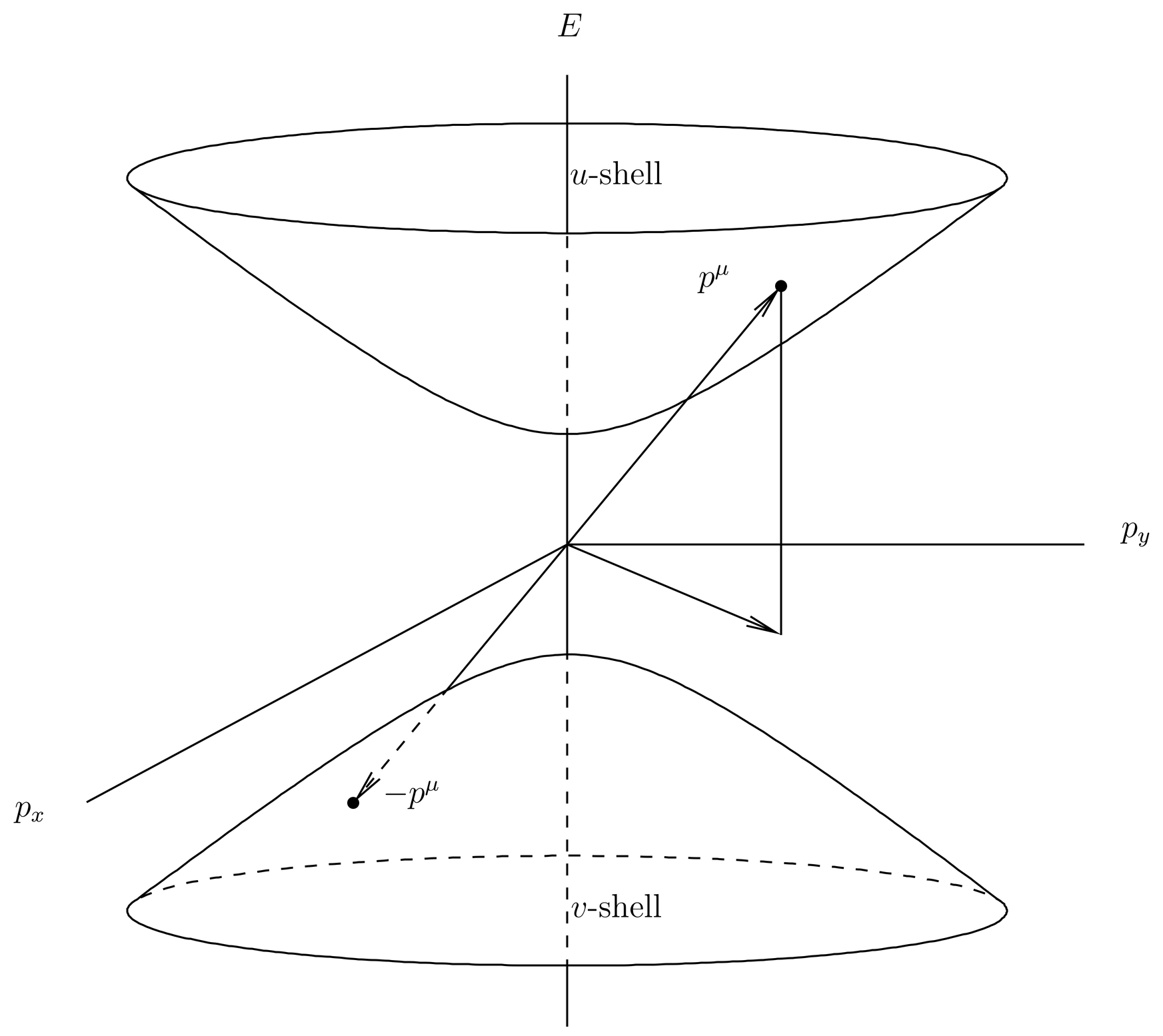
Figure 2:The forward and backward mass shells, the surfaces upon which , are illustrated, in 4-momentum space. Given a 3-momentum (illustrated in only two dimensions in the figure), we can erect the vertical in the direction, which intersects the forward mass shell at the 4-momentum . Directly opposite in 4-momentum space is the 4-momentum , on the backward mass shell. The -spinors are associated with the point and the -spinors with the point , so we call the forward mass shell the “-shell” and the backward one the “-shell.”
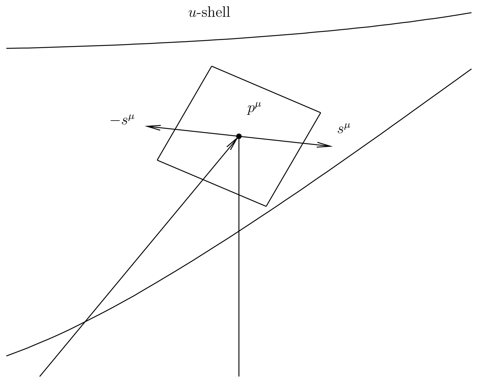
Figure 3:An enlarged view of the point with coordinates on the forward () mass shell. The “plane” (really a 3-dimensional space) tangent to the mass shell at this point contains vectors that are Minkowski orthogonal to , that is, they are purely spatial in the rest frame of the particle. Two opposite unit vectors and are chosen in this plane which specify the polarization of the spin.
Figure 3 contains a magnified picture of the point on the forward or - mass shell with coordinates . The plane tangent to the mass shell at the point is illustrated. In the diagram it is a plane, but really it is a 3-dimensional space. Vectors in this plane are Minkowski orthogonal to , so they represent 4-vectors that are purely spatial in the rest frame of the particle. Two unit vectors in this plane are illustrated, and , which represent two polarizations for the spin, and correspond to the spinors . A similar diagram applies on the backward or -shell. By convention, the spinor has 4-momentum and is polarized in the direction .
The Spinors and as Covariant Eigenspinors
The spinors and can be characterized in covariant notation as eigenspinors of certain Dirac matrices. First, the spinors and at rest are eigenspinors of , as we see from (14) and (6),
The eigenspaces of are 2-dimensional. But
so we have
Let us now boost these equations. Applying to (32), we find
where we use (42) in the second equality. Applying in a similar manner to (33) gives us altogether
The spinors and are eigenspinors of with eigenvalues and , respectively. Equations~(32) are special cases of (35) (for the particle at rest). Equations~(35) gives us covariant way of characterizing the -dependence of the spinors and .
Please note that (35) are purely spinor equations with no space-time dependence, and that involves the -number 4-vector , not the operator vector . The free particle Dirac equation in covariant form involves the operator 4-vector (see (8) or (13)),
When we apply this to a positive energy solution, we get
since just brings out from the exponent. When we apply it to a negative energy solution, we get
since brings out from the exponent. We have used (35) in the final step in both these results.
Equations~(35) can be used to construct projection operators , which when applied to an arbitrary spinor project out the positive and negative energy components. These are
and they satisfy
which says that they are complementary projectors. They also satisfy
which shows how they project out the positive and negative energy components of an arbitrary linear combination of positive and negative energy spinors.
One can also give a covariant way of characterizing the -dependence of and . It turns out that these spinors are eigenspinors of , and that projection operators can be constructed that project out the positive or negative components of spin along the spin vector . See Prob.~\prbrspdirac-1.
Orthonormality Relations for the Spinors and 
The spinors and satisfy two types of orthonormality relations, one the adjoint and the other the Hermitian. The adjoint relations are a bit easier to derive, so we present these first. The relations are
where takes on only two values, , so that is a polarization the same as or in the opposite direction in the rest frame. There is also the completeness relation,
where 1 represents the identity matrix, where the sum is taken over a polarization vector and its opposite, and the outer product of a column spinor times a row spinor is implied.
(42) may be proved as follows:
where we use (78). Thus is unchanged when referred to the rest frame. But
where we use (30). Equations.~(43) and (44) may be proved similarly, as may the completeness relation (45).
The Hermitian orthonormality relations involve a modified 4-vector , defined by , that is,
These are
where again, for given , the vector takes on only the two values, . The proofs of these relations will be left as an exercise.
The Gordon Decomposition of the Current
The next topic gives us some insight into why the velocity operator is a purely spin operator in the Dirac theory, in contrast to the nonrelativistic theory. The velocity operator appears in the Heisenberg equations of motion, in the probability current, and other places. See the discussion in Heisenberg Equations of Motion.
We will work with the covariant version of the Dirac equation for a particle interacting with an external electromagnetic field, (11). We write this equation in the form,
We multiply this on the left by by , which causes the current to appear on the right hand side,
The right hand side of this equation is real but the left hand side is not obviously so. To bring out the reality, we take the complex conjugate of (53), which, after the use of (79), can be written
We add these two together. The terms involving give
As for the terms involving the derivatives of , we use
(see (18) and (55)), to obtain
Altogether, we obtain
after dividing by .
(58) is the Gordon decomposition of the Dirac current. The first term is obviously a generalization of the Klein-Gordon current (see (27), with the addition of the interaction with an electromagnetic field. The Klein-Gordon current, in turn, is a relativistic generalization of the probability current for a spinless, nonrelativistic particle, given in (57). This term alone is called the convection current, since it involves only the purely spatial operator , which describes the state of motion of the particle. The second term in (58) is called the magnetization current, since it is the relativistic generalization of the magnetization current that was introduced in The Pauli Equation.
In summary, the Gordon decomposition of the current shows us that the velocity operator in the Dirac theory, a purely spin operator, corresponds to the entire current of the nonrelativistic theory, including the magnetization current. We may point out that the Dirac version of the classical force that a charged particle experiences in a magnetic field is , as shown by (41). That is, the magnetization current contributes to the force, which is what we would expect physically.
The Zitterbewegung
Other strange features of the Dirac velocity operator that were discussed in Heisenberg Equations of Motion included the fact that the velocity is not constant, even for a free particle, and the fact that the different components of the velocity do not commute with one other. We return now to the Heisenberg equations of motion, the subject of Heisenberg Equations of Motion, working for simplicity with the case of a free particle.
Specializing the results of Heisenberg Equations of Motion to the case of a free particle, we obtain the Heisenberg equations of motion for and , that is, , (we henceforth omit the hats on the momentum operator). As for , we work out the Heisenberg equations of motion as follows:
We write it this way because the anticommutator of with is easier to work out than the commutator. Using (8) we get the anticommutator,
Thus we have
What makes this equation easy to solve is the fact that both and are constants of motion. One way to solve an operator equation like (61) is to interpret all the quantities as -numbers, then to solve the -number equation as an ordinary differential equation, then to use that solution to guess the solution to the operator equation, which can be checked by back-substitution. In this case, the quantities and in the -number equation are taken as constants. Of course operators do not commute in general while -numbers do, so we can expect that the -number equation can be wrong by an ordering of operators, which we must take into account when making the guess. In this case the procedure is straightforward; (61) interpreted as a -number equation can be easily solved by Lagrange’s method of variation of parameters, and the solution makes it easy to guess the solution to the operator equation. In this way we find the solution to the Heisenberg equation of motion (61),
This can be checked by back substitution.
In this solution means the operator multiplied by the operator . It does not matter which order we do the multiplication, because and commute (otherwise the notation would be ambiguous). Also, we note that is defined because the spectrum of (see Figure 1) has an energy gap from to and does not include .
To interpret this equation we multiply through by to get the velocity operator,
We integrate this with respect to time, obtaining
the solution for the position operator in the Heisenberg picture.
The first term of (63), interpreted classically, is exactly the classical expression for the velocity as a function of the momentum in special relativity. See (39). It is, moreover, constant in time, as we expect for the velocity of a free particle in relativistic mechanics. We know, however, that the velocity does not commute with the Hamiltonian in the Dirac theory, so the velocity is not really a constant. The time dependence is contained in the second term in (63), which contains the factor .
To understand this time dependence better, we take the expectation value of (63) with respect to a state that contains mainly positive energy solutions of energy close to , that is, an essentially nonrelativistic state. This is all in the Heisenberg picture, so is the initial wave function. Then the Hamiltonian applied to this state brings out a quantity of order , and the operator behaves like the phase factor . This factor oscillates on a time scale of order , which is of order times smaller than the (already short) time scale in atomic units. See Table 1.
For we can replace the exponential by simply 1, and (63) and (64) become
On this time scale the expectation value of moves in a straight line. Also, since the eigenvalues of each component of are , the electron moves at a velocity comparable to the speed of light, so the distance covered in time , before the phase factor has a chance to change sign, is of order
that is, the Compton wavelength.
If the particle is essentially nonrelativistic then the the expectation value of first term in (63) is , so it is small in comparison to the second term. But on time scales , the second term averages to zero, while the integral of the first term continues to accumulate. Thus on longer time scales, we have
and the expectation value of the particle position follows a straight line at constant velocity, as we would expect from classical relativistic mechanics.
The rapid motion of the particle on a time scale of and a length scale of the Compton wavelength was first pointed out by Schr"odinger in 1930, who called it the Zitterbewegung, German for “jittering motion.” An interesting feature of the Zitterbewegung is that it is not present in a wave packet consisting solely of positive energy solutions. See Prob.~\prbrspdirac-5. The Zitterbewegung, when present, arises from the interference between the positive and negative energy solutions.
For this reason we may question if the negative energy solutions are real. Perhaps we should just declare them to be nonphysical, then we would not have to interpret them and the Zitterbewegung would go away.
Unfortunately, this does not work, for quite a few reasons. First of all, we can solve the Dirac equation for other problems besides the free particle. For example, the Dirac equation for the hydrogen atom is exactly solvable, and it gives positive energy solutions in good agreement with experiment, including the fine structure. These positive energy solutions can be expanded as linear combinations of free particle solutions, but the positive energy free particle solutions by themselves do not form a complete set. Thus, the expansion of (say) the ground state wave function of the Dirac hydrogen atom as a linear combination of free particle solutions will necessarily contain some negative energy components. In addition, the solution of the Dirac hydrogen atom also possesses negative energy solutions, and we have (at this point) no more physical interpretation for them than we do for the negative energy solutions for the free particle. But if we are going to declare them nonphysical, we now have a problem: Are we going to declare the negative energy free particle solutions nonphysical, or the negative energy hydrogen atom solutions? These two classes of negative energy solutions do not span the same subspace of the Dirac Hilbert space.
On the other hand, if we accept the negative energy free particle solutions, then we must have Zitterbewegung in any state that is a linear combination of both positive and negative free particle solutions. But we have just seen that the Dirac hydrogen atom wave functions are precisely such linear combinations. So does the Zitterbewegung exist in hydrogen? The answer is yes, it lies behind the Darwin term, as explained in The Hamiltonian. We will make a more careful analysis of the relation between the Darwin and other fine structure terms and the Dirac equation in a later set of notes, but for now we can see that there is no option to naively discard the negative energy solutions.
Ultimately we will see that the negative energy solutions of the free particle Dirac equation are related to positrons, the antiparticle of the electron, and that the Zitterbewegung is related to the fact that when an electron interacts with a potential, such as the potential of the nucleus in the hydrogen atom, there arises some finite amplitude for the formation of an electron-positron pair. That is, for brief periods of time, at least, there exist three particles instead of just one: two electrons and one positron. But in the early history of the Dirac equation, no one suspected the existence of antimatter, so these interpretations lay in the future.
Central Force Motion and Complete Sets of Commuting Observables
In the case of a central force potential the time-independent Dirac equation can be reduced to a pair of one-dimensional, first-order, coupled radial wave equations, a generalization of the single second-order radial wave equation that arises in the nonrelativistic theory (see (7) and (11) for the latter). In some cases the Dirac radial wave equations can be solved in terms of standard special functions of mathematical physics. The main example that we are interested in is the Coulomb potential, but part of the analysis applies to any central force problem so we treat that first. The Coulomb potential (for hydrogen-like atoms) is covered in Secs.~The Hydrogen Atom--18. For the rest of these notes we use natural units (), except at the end where we restore ordinary units when presenting results.
We seek the energy eigenvalues and eigenfunctions of the Dirac Hamiltonian in a central force potential, that is, we wish to solve
where
We identify the potential with in problems with electrostatic fields.
We appeal to the fine structure model of atoms (see 25. Fine Structure in Hydrogen and Alkali Atoms) for hints as to how to proceed, since this model incorporates relativistic effects to order , relative to nonrelativistic energies. We recall that a complete set of commuting observables in the fine structure model is . Of these, , and are commuting observables also in the relativistic (Dirac) problem, since commutes with the Hamiltonian (71). However, , as we find by a direct calculation of the commutator, so cannot be used as a member of the complete set in the relativistic theory and must be replaced by some other operator. In a moment we will see what the choices for this (fourth) operator are.
Accepting that and will be members of our complete set, we begin by looking for the most general eigenfunction of these with quantum numbers . We work in the Dirac-Pauli representation of the Dirac matrices, in which the matrices are block-diagonal,
We break the 4-component Dirac spinor into two 2-component Pauli spinors,
so that the action of the Dirac angular momentum on is equivalent to the action of two Pauli angular momenta acting separately on and . Thus the eigenfunctions of and in the Dirac theory are 4-component spinors in which both and are eigenfunctions of the Pauli operators and , with the same quantum numbers .
Eigenfunctions of in the Pauli theory are conveniently expressed in terms of spinor spherical harmonics, which are 2-component spinors defined over the unit sphere. We define them by
where for are the spin-up and spin-down spinors (the unit vectors in spin space), and where in the Clebsch-Gordan coefficient has the value . The spinor spherical harmonics are eigenfunctions of as well as and , with quantum number , which, for a given value of can take on only the values . Of course, is a half-integer, . We are seeing eigenfunctions of here because they arise when we construct eigenfunctions of and by the usual method of coupling , but since we do not expect to find energy eigenfunctions of the Dirac Hamiltonian that are also eigenfunctions of . In any case, the spin spherical harmonics are eigenfunctions of only as Pauli spinors, not as Dirac spinors.
The Clebsch-Gordan coefficients in (74) can be worked out by the method of Prob. Paragraph. These allow us to write out the explicit forms of the spin spherical harmonics,
where each and each is understood as a function of . We note that the spinor spherical harmonics are orthonormal,
We can now write down the most general 2-component eigenfunction of with quantum numbers . It must be a linear combination of for the two values , where each of the coefficients is allowed to be an arbitrary function of ,
From this it follows that the most general 4-component spinor that is an eigenfunction of the Dirac operators with eigenvalues is of the form,
where , , and are four arbitrary radial wave functions and where the upper and lower 2-component spinors have the same values. The radial wave functions will be determined by demanding that be an eigenfunction of the remaining members of our complete set of commuting observables.
The Fourth Observable and the Operator 
Now we can see some choices for the fourth observable in the complete set of the Dirac theory, the one that will replace in the fine structure model. The simplest choice is parity, which in the Dirac theory is discussed in Improper Lorentz Transformations and Parity. We write the Dirac parity operator as
where takes care of the spatial part of parity,
and where takes care of the spin part. The parity operator has an arbitrary ± sign (see Improper Lorentz Transformations and Parity), which we have chosen in (80) so as to make the intrinsic parity of the electron +1. In the case of 2-component (Pauli) spinors, the parity operator consists of alone, which takes into . See 21. Parity.
When we apply to the Dirac spinor (78) it brings out in each term, that is, . Thus the and terms acquire opposite signs, as do the and terms. But when we multiply the spinor by , the lower 2-component spinor acquires an additional phase of -1. Therefore if we require that the Dirac spinor (78) be an eigenstate of parity, then either , in which case the parity is , or else , in which case the parity is . We will write the simultaneous eigenfunctions of as
where the first and second spinors have parity and , respectively, where the arbitrary radial wave functions are now written as and and where for later convenience we have split off a factor of in the lower component. We see that indeed these spinors are not eigenfunctions of , which has a different value in the upper and lower components.
We have introduced a new quantum number in (81), which is related to the eigenvalue of a new operator . This operator serves as well as parity for creating a complete set, but it is not as obvious a choice. It is defined by
This is a scalar under spatial rotations so it commutes with . It also commutes with parity , that is, it is a true scalar, not a pseudoscalar.
The fact that it also commutes with follows from a straightforward but not very illuminating calculation. First note the commutator and the identity,
which follows from the definitions (11) and (108) and which implies
To compute we need the commutator,
which is expressed in terms of an anticommutator as shown. As for the latter, we migrate factors in the second term,
using (21). We continue to migrate factors in the first term in this expression,
since . This cancels the first term of the anticommutator in (85). As for the second term in (86), it is
which gives finally for the commutator (85),
The other commutators we need are and
so that on adding (89) and (90) and assembling the pieces we obtain .
In view of these commutators we will henceforth take as our complete set of commuting operators, although parity could be used in place of .
To obtain the spectrum of we first note that for the Dirac angular momentum we have
Next we look at the square of ,
We evaluate the first term of this result with the help of (152),
which is a little tricky, since is not zero, rather it is equivalent to the commutation relations . Thus we obtain
and when we apply to an eigenstate of with eigenvalue , it brings out . Therefore the eigenvalues of are .
To apply to the wave functions (81) we need the action of the Pauli operator on the spinor spherical harmonics. Since the Pauli angular momentum is given by , we have
which looks like (91) but is a Pauli, not a Dirac, operator. This implies
which in turn implies, for the two values ,
These show that if we apply the Pauli operator to the upper and lower components of the Dirac spinors (81), we bring out a factor of in one component and in the other. But then when we multiply by , the entire Dirac spinor acquires an overall factor, which is the eigenvalue of for the first spinor in (81) and for the second. Thus the eigenvalue of distinguishes the two spinors in (81). It is customary in the literature to denote the negative of the eigenvalue of by , which has the value for the first spinor in (81) and in the second. The extra minus sign is confusing, but we fear greater confusion if we change the convention. Table 1 summarizes the relations among , the parity, and the angular momentum quantum number attached to the upper and lower components of the Dirac spinors (81).
Table 1:Values of quantum number for upper and lower spinors and overall parity, as a function of , the eigenvalue of .
Recall that in the nonrelativistic limit, the upper 2-component spinor of the Dirac theory becomes the Pauli spinor of the nonrelativistic theory. See The Nonrelativistic Limit of the Dirac Equation. In the case of the Dirac spinors (81), we see that the quantum number of the nonrelativistic limit is the one labeled in Table 1, and that the radial wave function of the relativistic theory becomes of the nonrelativistic theory. The radial wave function is discussed in The Radial Schr"odinger Equation.
It is common in the literature to label the eigenfunctions of by rather than as we have done here, where refers to in Table 1. This has the advantage of labeling the solutions of the Dirac equation by the same quantum numbers that apply in the nonrelativistic limit, but of course it does not imply that the Dirac wave functions are eigenfunctions of .
The Action of 
(81) now gives us the simultaneous eigenfunctions of . When we demand that these also be eigenfunctions of we obtain equations that will determine the radial wave functions and . We substitute the spinors (81) into the Dirac equation, obtaining
where the upper sign refers to the first spinor (81) and the lower sign to the second. The corresponding values of are shown in Table 1.
This makes it evident that we will need to evaluate expressions of the form , where is some radial function. It is easier to evaluate (with instead of ), because it is only a multiplicative operator on the -space wave functions and not a differential operator. Moreover, once we have the latter we can obtain the former by using the identity,
where we use (152) and the fact that .
Therefore we turn our attention to evaluating
We see that under the action of the radial part of the wave function just gets multiplied by . As for the angular part, it will be desirable to expand it as a linear combination of spin spherical harmonics. To do this we freeze the radial coordinate and work with the Hilbert space of spinors over a sphere, in which the spin spherical harmonics form a complete orthonormal basis. We denote these in ket language by , where , , and . The radial coordinate can be regarded as just a constant for this part of the calculation.
In this notation we wish to evaluate
This sum simplifies. Since is a scalar under rotations generated by , it commutes with and hence with both and , so its matrix elements in the basis are diagonal in both and . Moreover it anticommutes with parity (it is a pseudoscalar, not a scalar), so it must map a state with quantum number into one with quantum number . This means that in the sum (101) can only take on the value , where if then . Thus the sum (101) reduces to a single term, which in the two cases can be written
where and are given by
But since is Hermitian, these imply . Finally, since , we see that is a phase factor, .
There is some effort in evaluating the final phase . A straightforward method is simply to apply the matrix in (100) to the spinors (75), noting that the components of the matrix can be written in terms of the 's for , as in (17). The product of 's can then be expressed in terms of single 's by means of the 3- formula, (72), and finally the result can be expanded in terms of spinor spherical harmonics. After some algebra along these lines, we find . We summarize the results by writing
where again if , then .
Now we divide both sides of (104) by and apply , using (99) and (96). We find
Writing this out for the two cases , we obtain
which is the desired action of on 2-component eigenfunctions of .
The Radial Wave Equations
Now we may substitute (106) into the Dirac equation (98). While we are at it we will express the radial wave functions , in terms of alternative radial wave functions and , defined by
which are just like the transformation (10) used in the nonrelativistic theory to create what we called version two of the radial wave equation.
The result is two coupled, 2-component equations equations for the upper and lower components of the Dirac spinor, from which the common spinor spherical harmonic can be canceled, leaving two coupled radial wave equations for and . These are
where as in (98) the upper sign corresponds to the first spinor (81) and the lower sign to the second. These equations can also be written in terms of the quantum number ,
where , as indicated in Table 1. These are the radial wave equations in the Dirac theory that replace version two of the radial wave equation, (11), in the Schr"odinger theory.
The nonrelativistic limit of these equations is obtained by the method of The Nonrelativistic Limit of the Dirac Equation. That is, we approximate so that the right hand side of (109) becomes , which allows that equation to be solved for in terms of . This is then substituted into (110) to eliminate and obtain an equation purely for . This turns out to be version two of the radial Schr"odinger equation, (11).
The Hydrogen Atom
We now specialize to the case for a hydrogen-like atom. We will solve the Dirac equation (70) for the bound states in this potential. Note that in natural units , so that is a dimensionless parameter of the problem. This parameter ranges from about for hydrogen to about for uranium and beyond, remaining, however, always less than unity for all known nuclei. As we will see, the ground state of the Dirac equation is a bound state only for , that is, , and becomes unbound for higher . This lends some interest to the question of whether nuclei with exist or could be made, even briefly. Note, however, that the potential is an idealization and that in the real world it must be modified at small radii because nuclei are not point charges. The corrections required for this become more important as increases. See Breaking the Extra Degeneracy and Prob. Paragraph.
Since the probability density in the Dirac theory is , the normalization integral for normalized bound states is
If we specialize this to Dirac wave functions of the form (81) and carry out the integral in spherical coordinates, we have
where we use (76). We see that a Dirac central force eigenfunction is normalizable if and only if both and are normalizable as one-dimensional wave functions on the interval .
We first look at the Dirac equation when is large, so that the potential energy and the terms that involve can be neglected. Then (109) become
or,
If these have oscillatory solutions that are not normalizable and cannot represent bound states. Likewise if the solutions are of the form , which are not normalizable. We see that the Dirac hydrogen-like atom has a continuous spectrum for , which corresponds to the positive energy, continuous spectrum of the nonrelativistic hydrogen atom. But the Dirac equation also possesses a continuous spectrum for , that is, it possesses negative energy solutions, just like the free particle.
Finally, if then the solutions go as
which are normalizable if we choose the minus sign. We see that bound states are possible only in the range , that is, , and that the eigenfunctions must behave asymptotically as .
We define a new radial variable,
so that the asymptotic behavior of the bound state wave functions will be . Then (109) become
where
Next we define new radial wave functions and , in which the asymptotic behavior has been stripped off,
which cause (117) to become
We examine the behavior of the solutions near . We assume that the dominant behavior of and when is small is and , respectively, for some powers and , where and . Then the left hand side of (120) is dominated by and the right hand side by . Therefore if the right hand side dominates, and we must have or . But this contradicts our assumption about the leading behavior, so we cannot have and we must have . A similar argument applied to (121) shows that we must have . Taken together, these imply . We see that both and begin with the same power .
It then follows that to leading order both sides of both (120) go as , and that the coefficients must satisfy
or
Thus, the determinant of the matrix must vanish, or,
Because the smallest value of is 1, we see that the exponent will be real for all as long as .
The case does not occur in real atoms, and even if it did, the potential would not be pure Coulomb because nuclei are not point charges. Nevertheless there is some interest in solving the problem anyway. We see that leads to purely imaginary exponents for small values of , which, as it turns out, produce wave functions that are oscillatory and not normalizable. Thus, the usual ground state of hydrogen would disappear as a bound state for such high values of , and be replaced by unbound states. This strange behavior for high is related to what is called the “supercritical vacuum,” and is properly understood by methods of quantum field theory. In a sense what happens is that for high the electric field becomes strong enough to pull electron-positron pairs out of the vacuum, and thus a multiparticle situation is created.
Similar effects occur in a square well potential, if it is deep enough. You would think that the deeper the well gets, the more tightly bound the electron would be, but in the Dirac equation that is not so, since for deep enough wells we start to get unbound solutions. This effect is related to what is called the “Klein paradox,” another one of the puzzling aspects of the Dirac equation, when treated as the wave equation for a single, relativistic particle. In these notes we assume , which means that is real for all .
Now it turns out that we can reject the minus sign in (124) on grounds of the regularity of the wave function. If we require that the amount of probability in a region near be finite, then the integral
must be finite for some . But this implies , or . If we demand in addition that the expectation value of the potential energy term be finite, then we obtain , or . These regularity conditions are discussed in greater detail by W. Greiner, Relativistic Quantum Mechanics. We henceforth take only the positive root for in (124).
If is small then is approximately , an integer, but with a small negative correction. With the correction is not an integer, so the wave function behaves as a fractional power of near the origin. In the case , is a fraction less than 1, which means that the wave functions and (see (107) go like a small negative power of near the origin. That is, they diverge at , unlike the nonrelativistic solution, which is regular there. In spite of the divergence, the net probability in a neighborhood of the origin is finite, as is the expectation value of the potential, as noted above.
Recursion Relations and Energy Levels
We now write and as power series,
and substitute these into (120). By equating coefficients of the different powers of we obtain recursion relations for the coefficients and . These are conveniently written in matrix--vector form,
where
and
It is understood that for . In the following we will use letters , , etc., at the end of the alphabet for 2-component vectors, and those near the beginning, , , etc., for scalars, for example, and are the components of .
Setting in (127) we obtain , which is (123). Since this implies , which as shown above determines . As for , it is any nonzero vector in the one-dimensional kernel of . For the matrices are nonsingular, since
so we can write the recursion relation as
The matrix is also singular. We pay special attention to its image, a one-dimensional space spanned by
Vector is an eigenvector of with eigenvalue 1,
The kernel of is conveniently handled with the adjoint (or adjugate) of . If is any matrix, then the adjoint is defined by
so that . Thus and maps any vector into a vector in the kernel of . It is convenient to choose
In the following we will need , which must be a multiple of . Using (128) and (135), we find
where
Also, for we write
Now to apply the recursion relation (131) for we must evaluate
so that
Iterating the recursion relation in a similar manner, we obtain
If is not an integer then as gets large the coefficient in front of approaches , so that the series for both and behave like . This overwhelms the factor of that we have stripped off, making both and diverges as as . These solutions are not normalizable and must be rejected. We conclude that must be a nonnegative integer, , with . Then for , and both and are polynomials in of degree . These are dominated at large by , so that the wave functions are normalizable and acceptable as bound states.
Now since
(138) becomes
which we solve for to obtain,
where we have restored ordinary units. These are the energy eigenvalues of the bound states of the Dirac hydrogen atom; they are functions of the two quantum numbers, and . The bound state energies are all positive and lie in the interval .
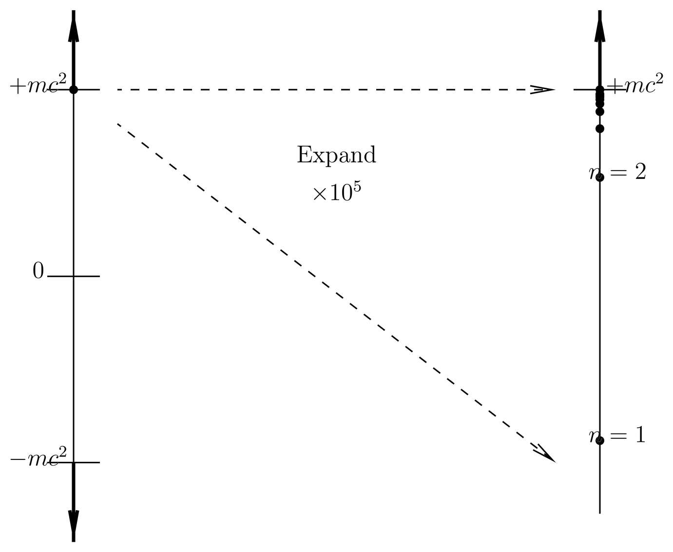
Figure 4:The energy spectrum of the Dirac hydrogen atom, here illustrated for . The usual hydrogen ground state lies 13.6 eV below the rest mass-energy, , and the usual unbound states of the Schr"odinger theory lie in a continuum above . However, there also exists another continuum of unbound (negative energy) states with .
To connect these quantum numbers with those of the nonrelativistic hydrogen atom, we expand in powers of . For this we only need to lowest order,
so that
where (see Table 2) is the effective Bohr radius and where we set
which is identified with the usual principal quantum number of the nonrelativistic problem. To second order in , the Dirac energy levels are the rest-mass-energy of the electron, shifted downward by the binding energies of the Schr"odinger theory in the electrostatic model.
Expressed in terms of instead of , (144) becomes the Dirac hydrogen energy levels as cited in (57). As discussed in 25. Fine Structure in Hydrogen and Alkali Atoms, the energy levels (144), when expanded to fourth order in , yield all the fine structure corrections obtained by perturbation theory in those notes. This means that the Dirac equation automatically incorporates the spin-orbit corrections, including the factor of due to Thomas precession, as well as the not-so-obvious Darwin term. All this complexity in the Schr"odinger-Pauli theory is contained in the simple equation (13). The entire spectrum of the Dirac hydrogen atom is illustrated in Figure 4, including the two continua of unbound states with and .
Energy Eigenfunctions
It is now straightforward to work out the energy eigenfunctions. We combine (119), (126), (129) and (141) with to obtain
where we use Abramowitz and Stegun, Handbook of Mathematical Functions, Eq.~(22.3.9), for the definition of the associated Laguerre polynomials. In the present context that definition can be written,
Also, the 2-vectors and are given by (132) and (135). In these formulas it is necessary to use gamma functions instead of factorials, because the upper index of the Laguerre polynomials () is not an integer.
To explore the nonrelativistic limit it is convenient to use the identities,
of which the first is easily derived from the definition (149) and the second is Abramowitz and Stegun, Eq.~(22.8.6) (and which is also easily derived from the definition). Then we have two expressions for the radial wave functions,
where we drop the constant prefactors seen on the right in (148) since at this point we are not interested in the normalization. The two forms of the solution (151) are useful for taking the nonrelativistic limit, in which we expand everything to lowest order in . The form (151) is useful when , in which case the second term dominates and produces to leading order in , which is the nonrelativistic wave function (see (16); and the form (151) is useful when in which case the second term again dominates and produces the same nonrelativistic wave function.
The normalization of the Dirac wave functions may also be obtained in closed form; it may be found in the references.
Problems
Problem 1.
Show that and are eigenspinors of with eigenvalue . Thus we can define spin projectors,
which project out the positive and negative spin components of an arbitrary 4-spinor of a free particle. As far as the negative energy spinors are concerned, notice that these project out the components whose labels are and , while the labels are the negatives of the spin eigenvalues.
Problem 2.
The orthonormality and completeness relations (\eqr\cn.41), (\eqr\cn.42) and (\eqr\cn.46) will be important in future applications.
(a) Prove (43), (44) and (45).
(b) Prove (49). It may help to note that the matrix for a pure boost is Hermitian, and that .
Problem 3.
Show that
that is, the positive and negative energy projectors are the first and second terms in (45), respectively. As in that equation, the summation is taken over two spin vectors that point in opposite directions in the rest frame.
Problem 4.
In Sec.~\secr\dirac.9 we carried out a nonrelativistic approximation on the Dirac equation. The essence of the approximation was Eq.~(\eqr\dirac.46), which expresses the lower two components of the Dirac spinor in terms of the upper two components . Notice that this equation has a relative error of order , when the solution of the Dirac equation has an energy which is plus a small (nonrelativistic) correction of order .
Apply this approximation to the Dirac current to get the probability density and probability current in the Pauli theory, to order . See if the answer includes a magnetization current. See The Pauli Equation.
Problem 5.
An arbitrary free particle solution of the Dirac equation is a linear combination of the positive and negative energy solutions, which we can write as
where and are expansion coefficients. We write these as if they depend on two 4-vectors and , but the notation is like the dependence of and , that is, the 4-vector is really a function of the 3-momentum (the variable of integration) and is taken over only two opposite unit vectors in the rest frame. This wave function is in the Schr"odinger picture, since the explicit time-dependence is given.
Compute the expectation value of the velocity operator to get , and show that it is independent of and contains no Zitterbewegung if the wave packet consists purely of positive energy solutions (that is, if ).
Problem 6.
Consider a Dirac electron () in a uniform magnetic field, . Choose the gauge,
which is translationally invariant in the -direction. This means that will be a constant of the motion (although you must distinguish between the kinetic and canonical momentum).
Here is some background on the nonrelativistic problem, which will save you some time. Ignore the spin and the motion in the -direction, for simplicity. Then the Schr"odinger equation is
Here we put hats on the momentum operators to distinguish them from the corresponding eigenvalues (where relevant), which are -numbers. For example, . Also, we define
Then the wave equation (156) is separable, and has the solution,
where is the eigenvalue of , where
and where is the usual, normalized Hermite function for the one-dimensional harmonic oscillator with frequency ,
Here is the usual Hermite polynomial, defined by (46). The energy eigenvalue for the eigenfunction (158) is
where is the Landau level. The energy is independent of the quantum number . The wave function is like a ridge in the - plane, centered on (i.e., on ), and running in the -direction.
(a) Solve the Dirac equation for the relativistic electron in the same magnetic field. This time you must include the -motion and the spin. Express the energy in terms of the quantum numbers . Write out explicitly a complete set of positive energy solutions as 4-component spinors. You need not normalize these solutions, and you may ignore the negative energy solutions.
(b) Consider the motion of a Dirac electron in the field,
where . The solution of the Dirac equation for this problem can be obtained from the solution to part (a) by using the transformation law (26). Find matrices and which will cause to be the solution in the field (162) if is the solution in the purely magnetic field of part (a). You will also need to find a relation between and . You need not write out the solution explicitly, but do find the energy eigenvalues in terms of the same quantum numbers as in part (a).