10. Charged Particles in Magnetic Fields
Introduction
An introduction to the quantum mechanics of charged particles in magnetic fields was given in 05. Time Evolution in Quantum Mechanics. In these notes we examine several problems involving charged particles in magnetic fields.
One of the issues that will be of most interest to us is the role of the magnetic vector potential in quantum mechanics. In classical mechanics and classical electromagnetic theory, one could say that is unnecessary, since both the equations of particle motion (18) and Maxwell’s equations are expressed purely in terms of and . Moreover, and are physical in the sense that they can be measured, while is not. One can construct devices that measure both and , but there is no such thing as an -meter. One can say that contains a physical element (because can be computed from it), but it also contains a nonphysical element (the part of that changes under a gauge transformation). In other words, is partly conventional (what we call the gauge convention).
Similar considerations apply to , the scalar potential, although not so dramatically as with the vector potential. There is no such thing as a -meter. It is true that there are volt meters, but they have two wires, and measure the relative potential between two points. Moreover, the potential difference is only meaningful in the electrostatic approximation.
When we turn to quantum mechanics, however, we are struck by the fact that the Schr"odinger equation, as a differential equation in , necessarily involves the vector potential. Moreover, the wave function is gauge-dependent (see Gauge Transformations in Quantum Mechanics). Does this mean that the vector potential has a direct physical significance in quantum mechanics? That is, are there physical effects in quantum mechanics that depend on the vector potential, that cannot be expressed in terms of alone?
The answer is no, a gauge convention remains just a convention in quantum mechanics, just as it is in classical mechanics. But quantum mechanics reveals that magnetic fields can have nonlocal effects, that is, a magnetic field in one region of space can have an effect on charged particles in another region of space where there is no magnetic field. These effects are expressed through the vector potential, while at the same time remaining gauge-invariant. This nonlocality is seen perhaps most clearly in the Aharanov-Bohm effect. Similar nonlocal effects occur in time-dependent electric fields.
We begin with some generalities on velocity operators, and then turn to the problem of a charged particle in a uniform magnetic field, a problem of great importance in condensed matter physics, astrophysics and elsewhere. Next we treat the Aharonov-Bohm effect, which reveals a kind of nonlocality in quantum mechanics that challenges our understanding of the meaning of the wave function. It does not, however, contradict any of the principles of quantum mechanics. Finally, we present Dirac’s analysis of the magnetic monopole, which leads to an explanation of the quantization of electric charge.
Velocity Operators
The Hamiltonian for a particle of mass and charge in an electromagnetic field is given in (73), which we reproduce here:
where the potentials and are related to and by (70). The momentum appearing in this Hamiltonian is the canonical momentum. In classical mechanics, the velocity of the particle is given in terms of the canonical momentum by
We adopt this formula also in quantum mechanics, and interpret as a vector of operators. The same definition of velocity arises when applying the Heisenberg equations of motion to the Hamiltonian (1), that is, (see Prob. Paragraph). In terms of the velocity operators, the Hamiltonian takes on the simple form,
This reveals the physical meaning of more clearly than (1), that is, the first major term of (1) is just the kinetic energy of the particle.
But the Hamiltonian in the form (3) raises a new question. If this is supposed to be the Hamiltonian for a particle in a magnetic field, why does the magnetic field (or even , from which can be computed) not appear in it? The same Hamiltonian would apply even if were zero, but obviously the physics would not be the same.
The answer is that the magnetic field is hiding in the commutators of the velocity operators, which do appear in the Hamiltonian. The components of velocity do not commute with one another, in general. Using the definition (2) and the commutators
(see Prob. Paragraph), we find
where
The antisymmetric tensor contains the components of the magnetic field,
Putting this together, we have
We also note the commutators,
The velocity commutators (8) are proportional to the components of the magnetic field. Notice that this result holds regardless of the nature of the magnetic field (nonuniform, time-dependent, etc), with or without an electric field. If the magnetic field vanishes, then the components of velocity commute with one another, as is obvious since in that case , and since .
The Uniform Magnetic Field. Classical Motion
We now consider the case , where is a constant (independent of space and time). We also assume the particle is an electron, with charge . In the case of a positive particle the direction of motion changes as do the signs in various formulas.
The classical equations of motion are
where is the velocity and the acceleration. These can also be written,
where
is the frequency of the orbital gyration of the electron (the gyrofrequency). We write out (11) in components,
(15) shows that is a constant, in fact, the motion in the -direction is that of a free particle in one dimension,
Next we integrate (13) and (14) once in time and write the result as
where and are constants of integration. Solving these for and , we have
We will interpret and momentarily.
Now define and , so that and . Then the equations of motion (17) become
The solution is
where we sum the exponential power series of matrices as in Prob. Paragraph(b). The final matrix is a rotation in the counterclockwise direction in the - plane by angle .
Now using , , we see that the orbit in the - plane is a circle centered on , as illustrated in Figure 1. Taking into account the motion (16) in the -direction, we see that overall the orbit in three-dimensional space is a helix. The particle moves on a circle parallel to the - plane, which itself is moving uniformly in the -direction with velocity . The center of the circle is called the guiding center. The guiding center coordinates are .
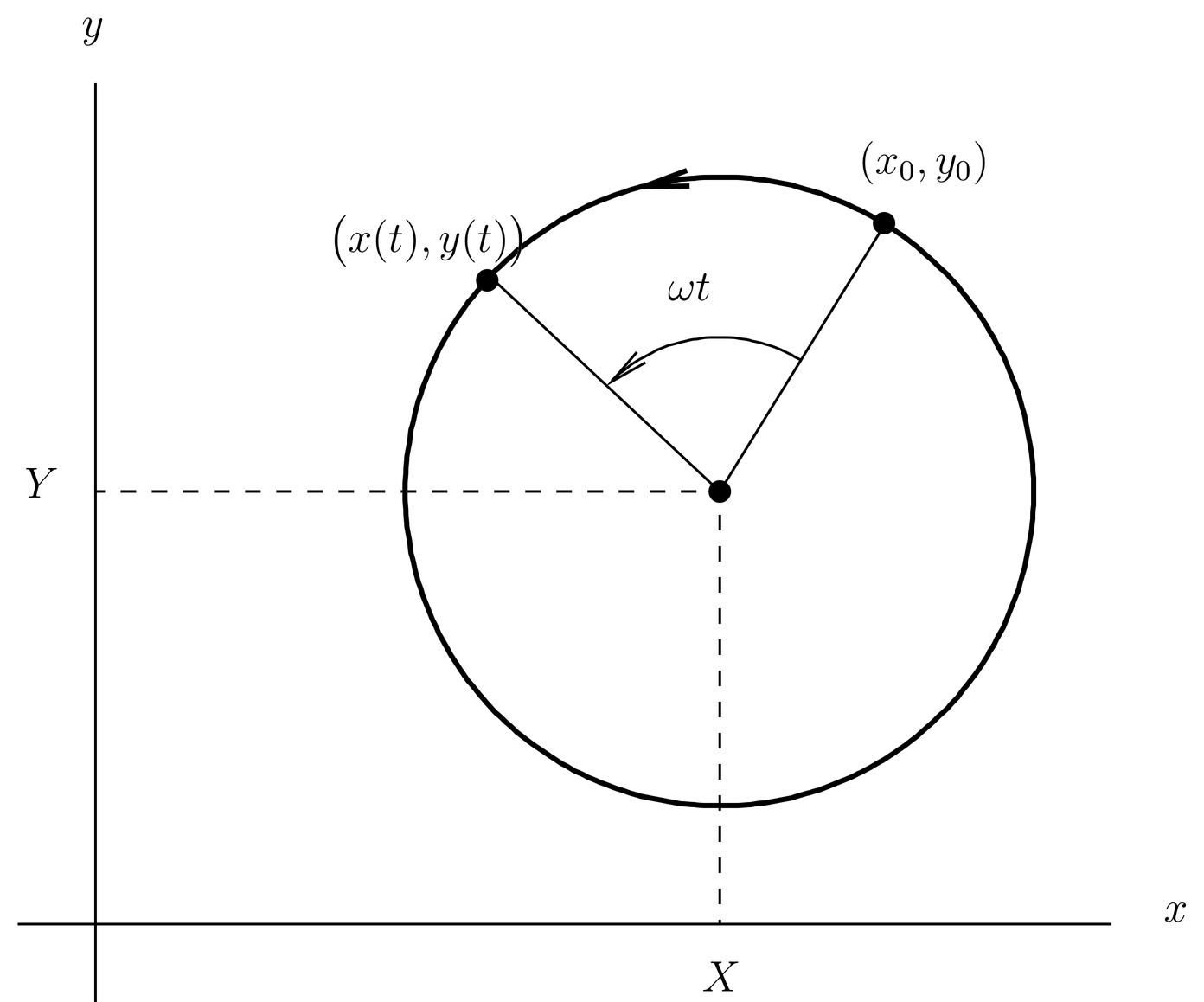
Figure 1:The classical motion of an electron in the - plane in a uniform magnetic field . and are the coordinates of the guiding center.
The Energy Spectrum
Now we turn to the quantum problem. First we shall determine the energy spectrum (that is, the energy eigenvalues). For simplicity, we ignore the spin of the electron. This is not a good approximation, because when the spin is included, the energy levels are rather different from what we find here. See Prob. Paragraph. We do it anyway, because it is easy to include the spin once we have solved the spinless problem, and we wish to address one issue at a time. The energy of the particle is something that can be measured, and so must be gauge-invariant. Therefore there must be a way of finding the energy eigenvalues in a gauge-invariant manner, that is, without committing ourselves to a gauge convention for . We will see that this is true.
The quantum Hamiltonian, expressed in terms of velocity variables, is given by (3) with ,
The energy is purely kinetic, and we have broken it into its parallel and perpendicular parts (that is, parallel to and in the - plane). Since and , the commutators (8) become
where is the frequency (12) of the classical motion. We see immediately that , so and possess a simultaneous eigenbasis, which is an eigenbasis of .
Our strategy for analyzing is to borrow definitions of interesting operators from the classical solution and to explore their properties. The most interesting operators for the perpendicular motion are , , and . The most interesting operators for the parallel motion are . We borrow the classical definitions of , (18), and reinterpret them as operator equations that define in terms of the position and velocity operators for the electron.
The commutator of the guiding center coordinates is
where we use (9) and (22). Similarly we calculate the other commutators among the operators . The results are summarized in Table 1.
Table 1:Commutators among various operators. The commutator in the table is , where is the operator labeling the row and is the operator labeling the column. The table is antisymmetric.
0 | 0 | 0 | 0 | 0 | ||
0 | 0 | 0 | 0 | 0 | ||
0 | 0 | 0 | 0 | 0 | ||
0 | 0 | 0 | 0 | 0 | ||
0 | 0 | 0 | 0 | 0 | ||
0 | 0 | 0 | 0 | 0 |
The table shows that to within constant factors, the set of operators forms a set of three canonically conjugate pairs of operators, that is, operators that satisfy the Heisenberg-Born commutation relations (74). To bring this out more clearly we define new operators , , by
so that
By working with variables of obvious physical importance, we have found a “canonical transformation,” that is, a transformation that preserves the canonical commutation relations. (See Canonical Transformations for canonical transformations in classical mechanics.)
Now we express in terms of these new variables, substituting (24) into (21). We find
The perpendicular kinetic energy appears as a harmonic oscillator, while the parallel kinetic energy appears as a one-dimensional free particle. The eigenvalues of are immediate; they are
We know this because Dirac’s derivation of the energy levels of the harmonic oscillator in Dirac’s Algebraic Method for the Eigenvalues depends only on the commutation relations of the operators and , which are reproduced here by operators and . The quantized energy levels of the perpendicular kinetic energy are called Landau levels.
(A note for the mathematically inclined. Technically, Dirac’s derivation also involves an assumption of the irreducibility of the representation of the commutation relations, which amounts to making certain assumptions of nondegeneracy. The consequences of this assumption, both in the case of the harmonic oscillator and in the problem of the particle in a magnetic field, are obvious physically and on a first pass need not be belabored.)
As for the eigenvalues of , they are those of a free particle in one dimension, that is, the spectrum is continuous with . Overall, the energy is
where now is an eigenvalue (a -number) of the operator , which has the spectrum .
The Hamiltonian (26) is unusual because it does not depend on , which are essentially the guiding center coordinates . It would not be unusual to find a Hamiltonian that was independent of one of the coordinates, in which case the conjugate momentum would be a conserved quantity. But in this case neither the coordinate nor the conjugate momentum appears, so they are both conserved. This makes sense physically, because classically the energy does not depend on where the circle is located in the - plane, and moreover both and are constants of motion.
The Hamiltonian in (26) does not look exactly like the standard Hamiltonian for a mechanical harmonic oscillator,
To bring out the relation between the two, we set
which is a canonical transformation preserving the fundamental commutation relations. It causes the Hamiltonian (29) to become
after dropping the primes. This has the same form as in (26).
We have succeeded in obtaining the energy levels of the electron moving in a uniform magnetic field by gauge-invariant means. That is, we never had to work with gauge-dependent quantities, such as or . It makes sense that we can do this, because the energy levels are experimentally measurable, and must be gauge-invariant.
The Energy Eigenfunctions
Wave functions in the presence of a magnetic field are gauge-dependent, as we have seen in Gauge Transformations in Quantum Mechanics, so we will have to choose a gauge convention for before we can find the energy eigenfunctions. One way to do this is to choose a gauge and then attempt to separate the Schr"odinger equation in some coordinate system. It turns out that if the gauge chosen has the right symmetry, then the time-independent Schr"odinger equation is separable in some coordinate system. In general, separability works when the system has some symmetry, although this is not completely obvious in the actual procedure.
The following method is more clear. Instead of focusing on the separation of the Schr"odinger equation, we look for a complete set of commuting observables for the Hamiltonian (21). In the following we put hats on the operators to distinguish from the corresponding -numbers , where . For other operators this distinction will not be necessary so we will omit the hats.
As we have already noted, and commute with each other and with , so we can take , or, better, as a pair of commuting operators. Recall that . But these operators do not form a complete set because the first degree of freedom , or, equivalently, the guiding center coordinates , are not represented. But since any function of commutes with any function of and , we can take any function of , or, equivalently, , as the third operator.
The fact that there is more than one way to choose the complete set of commuting observables means that the energy eigenfunctions are degenerate, and there is more than one way of choosing an orthonormal basis in the degenerate eigenspaces. Such freedom arises because the motion of a charged particle in a uniform magnetic field is a highly symmetrical problem. In particular, it is clear that the magnetic field is invariant under translations in the -, -, and -directions, as well as under rotations about the -axis. If we add further physical effects (for example, an electric field), then some of this symmetry is broken and the set of choices for a complete set of commuting observables narrows. For now we will take the third operator to be , or, equivalently, , which is probably the simplest choice. Thus we will be interested in finding the simultaneous eigenfunctions of .
Since and are simpler than , we find their eigenfunctions first. We start with , for which we wish to solve
where we use and (2). This equation is hard to solve because of the presence of . Can we choose a gauge so that ? We write out in components,
and we notice that if then and are independent of ,
This means that the entire vector potential is independent of , that is, it is invariant under displacements in the -direction. This is obviously one of the symmetries of the magnetic field , which with the choice is reproduced by the vector potential.
Since , we have
so henceforth we will write simply for , and similarly for the eigenvalue . Then (33) becomes
or,
where is an arbitrary function of . The wave function is a free particle solution in the -direction.
We determine by requiring that be an eigenfunction also of and . We start with , for which the eigenvalue-eigenfunction problem is
where is given by (38). But since the operator does not involve the coordinate , we can cancel the factor of , and we have
We simplify this equation by choosing to cancel the , that is,
or,
This is consistent with (34) if , so in effect we have now chosen the gauge,
This vector potential is invariant under translations in the - and - directions, but not the -direction. Of course the magnetic field is invariant under translations in all three directions. We see that overall, the vector potential has less symmetry than the magnetic field .
(41) now simplifies to
or,
where is an arbitrary function of . We now have a simultaneous eigenfunction of and .
We determine by requiring that also be an eigenfunction of , that is, we solve . But since does not involve the -coordinate, we can cancel the factor and work with
or,
But now brings down a factor , so we can cancel the phase factor and we have an equation purely in the coordinate ,
This is the equation of a harmonic oscillator, with origin shifted to . The energies are , which we knew already, and the eigenfunctions are
where are the energy eigenfunctions of the usual harmonic oscillator [see (48)]. Overall, the simultaneous eigenfunction of with quantum numbers is
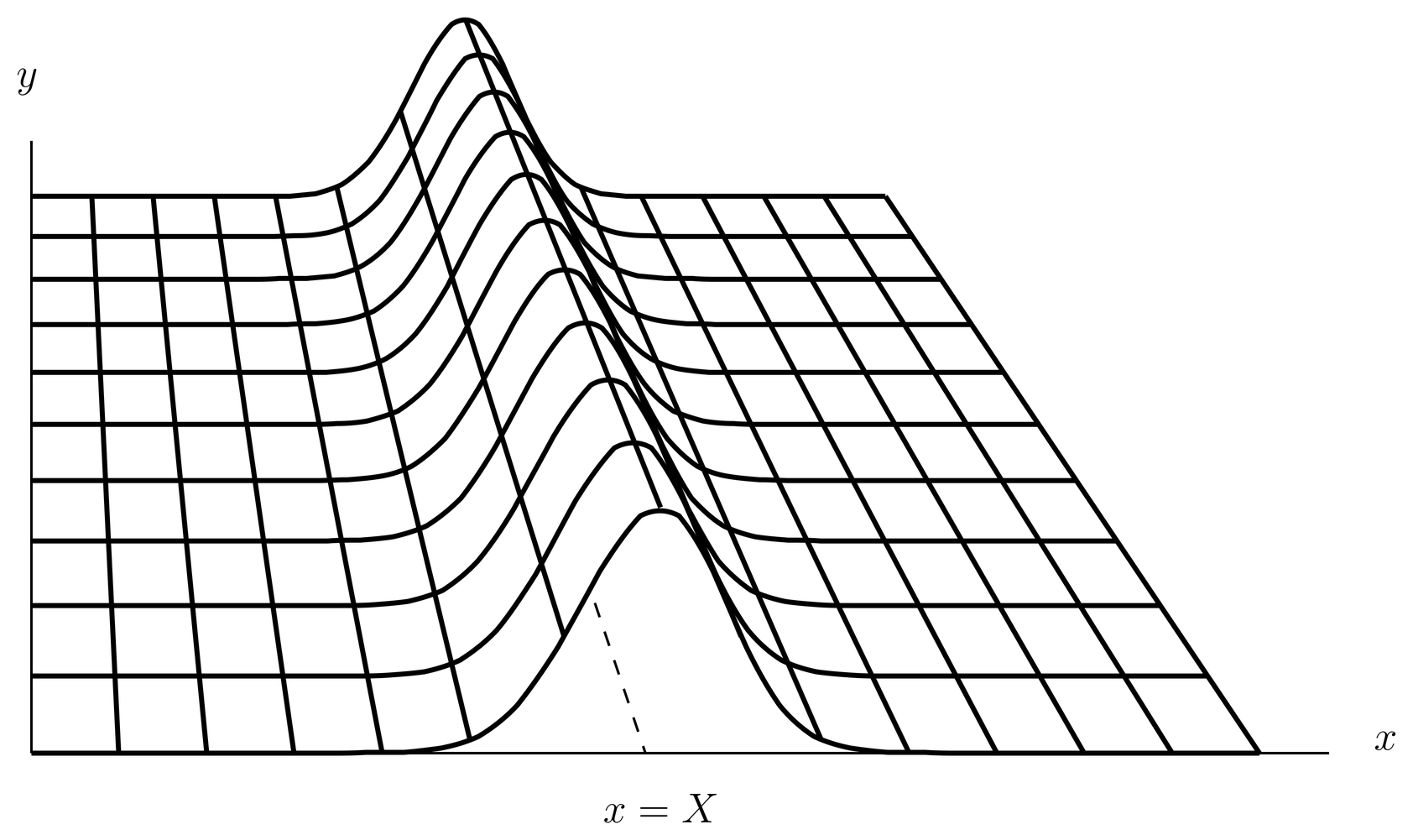
Figure 2:Plot of in the - plane for . Vertical direction is .
The probability density for the Landau ground state () in the - plane is plotted in Figure 2. Squaring the wave function gets rid of the phase factors in (53), and allows us to plot a real function. The result is a “Gaussian mountain range” that is centered on the line . Notice that the wave function does not look at all like the classical solution; that is because we have constructed an eigenfunction of , the -component of the guiding center position. But since and do not commute, the value of is completely undetermined. That is the reason the mountain range extends to infinity in the -direction.
We could have chosen instead of as the third observable (in addition to and ) to form a complete set, but the simultaneous eigenfunctions of that set would have mountain ranges extending out to infinity in the -direction. These features are a consequence of the nonvanishing commutator . The energy eigenfunction would still not look much like the classical orbits, in this case in effect because the classical orbit is smeared in the -direction.
Another possibility is to choose the -component of angular momentum as the third observable. This is explored in Prob.~\prbrmagfield-1. Does this produce wave functions that look more like the classical orbit? Unfortunately, no, because an eigenstate of must be completely indeterminate in the conjugate angle . It is as if the classical solution is smeared out by rotating it about the -axis. Remember that the classical orbit is a circle, but it is centered on , not the origin in general. So when the classical circular orbit is smeared around in , it creates an annular ring around the origin, which is where the eigenfunctions of are concentrated.
Can we find energy eigenfunctions that do look like the classical orbits? Yes, it turns out that we want to use a coherent state in the and operators. These are eigenfunctions of not only and but also of the annihilation operator proportional to . These are not eigenstates of complete sets of commuting observables, because the annihilation operator is not Hermitian and so is not an observable. But the energy eigenfunctions in this representation do resemble rather closely the classical orbits, that is, circles centered on the guiding center position (actually the expectation values of the operators , , as usual with coherent states). The use of coherent states in the motion of a charged particle in a uniform magnetic field is explored in Prob.~\prbrmagfield-4.
One final comment. In most of the literature the energy eigenfunctions (53) would be described as the “solution in the gauge ” [the gauge (44)]. This is because if we use the gauge (44) in the three-dimensional Schr"odinger equation, then it is separable in rectangular coordinates and the solution is (53). But it would be better to call (53) “the energy eigenfunctions that are also eigenfunctions of and ,” which is essentially what we have done here, since once the solution is obtained (by any means) we can perform a gauge transformation on it, as described in Gauge Transformations in Quantum Mechanics, and put it into any gauge we want. The gauge transformation will change the phase of the wave function but not , so Figure 2 does not change, nor does the physics that explains the mountain range in the -direction. The usual terminology confuses the gauge which causes the Schr"odinger equation to be separable with the gauge in terms of which the wave function is expressed. If we consider a class of wave functions that are related by gauge transformations as being physically equivalent, then the physics of the solution is determined by the complete set of commuting observables, not the gauge.
The Flux Quantum
Although the and coordinates of the particle are commuting operators, as we have seen the and coordinates of the guiding center are not. Thus, the guiding center - plane is more like a phase space than a configuration space. The same can be said for the - plane.
Let us consider a region of the guiding center plane with an area of one Planck cell. See Planck Cells and Classical Statistical Mechanics for a discussion of Planck cells. Measured in terms of the variables and the area is . But this can be expressed in terms of the guiding center coordinates through (24),
or,
where is Planck’s original constant. This is the amount of flux passing through a single Planck cell of the guiding center plane. It indicates how much area of the guiding center plane is occupied by a single quantum state.
The quantity on the right hand side is a natural unit of magnetic flux, called a “flux quantum.” The name is somewhat inappropriate, because magnetic flux is not quantized---there is no rule that magnetic flux must come in integer multiples of a flux quantum. Nevertheless, the flux quantum is a unit that appears in many problems involving magnetic fields.
For example, two-dimensional electron systems are common in condensed matter physics, when electrons are trapped in the -direction by some potential, for example, at the interface between two media. Then if a magnetic field is applied perpendicular to the interface, the electrons occupy various Landau levels.
Naturally a realistic two-dimensional system like this does not extend to infinity but rather is confined to a finite area in the - plane by the size of the sample. If we fill up electron states starting from the ground state and increasing in energy, as we must if we want the ground state of a multielectron system, then how many electrons in the two-dimensional system can occupy the Landau ground state? The answer is the area of the sample divided by the area shown in (55), times two to account for the electron spin. That is, it is twice the number of flux quanta in the flux intercepted by the whole sample. After this, successive electrons enter the first Landau level until it is filled, etc.
If now we change the magnetic field, the number of electrons contained in each Landau level changes. If we increase the magnetic field then the ground Landau level can hold more electrons, so electrons from the first Landau level move down into the ground Landau level, etc. Conversely if we lower the magnetic field. (This is assuming the system remains in the collective ground state as the magnetic field is changed.) The physics described here lies behind the de Haas-van Alphen effect, which refers to the fact that the magnetization of a bulk sample is a periodic function of the magnetic field, under the right circumstances.
The Aharanov-Bohm Effect
We now take up the Aharanov-Bohm effect, which concerns the quantum mechanics of a charged particle in the field of a long solenoid. The analysis leads to further insight into the role of the vector potential in quantum mechanics, as well as the surprising conclusion that magnetic fields in one region of space can have an effect on charged particles in another region where the magnetic field is zero.
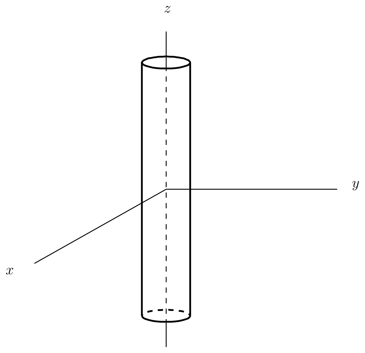
Figure 3:A long solenoid is centered on the -axis.
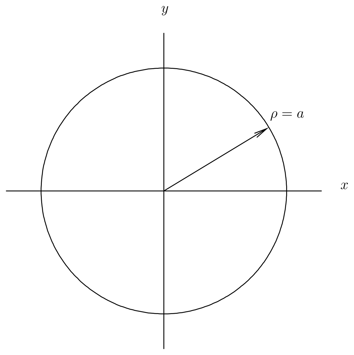
Figure 4:Cross of the solenoid. The radius in the - plane is .
The long solenoid is a simple problem in magnetostatics. We center the solenoid on the -axis, as shown in Figure 3. It has a circular cross in the - plane, as shown in Figure 4, with radius , where
The magnetic field is uniform in the -direction inside the solenoid and zero outside,
as illustrated in Figure 5.
To obtain the vector potential we assume it is in the -direction, , and then we integrate in the counterclockwise direction around a circle of radius in the - plane, centered on the -axis. We allow the circle to be either inside or outside the solenoid. The integral is the magnetic flux captured by the circle, that is,
or,
The magnetic field and vector potential are plotted in Figs.~Figure 5 and Figure 6. The magnetic field has a discontinuity at because of the surface current in the solenoid, but the vector potetial is continuous there. Note especially that the vector potential is nonzero in the exterior region where .
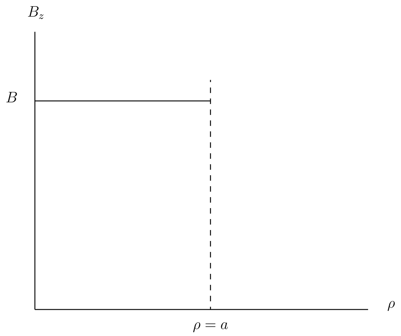
Figure 5:The magnetic field is uniform inside the solenoid and zero outside.
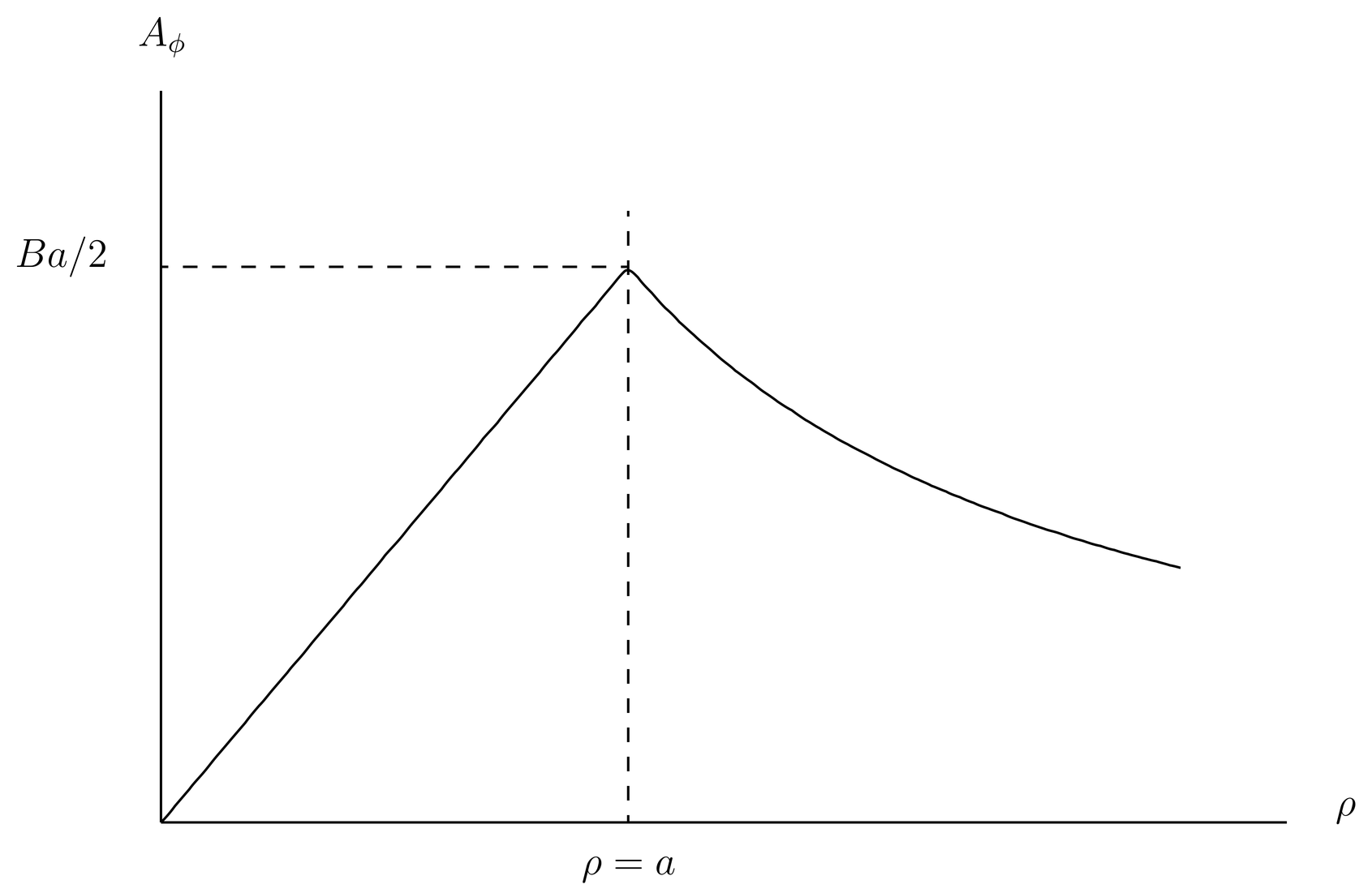
Figure 6:The vector potential is continuous at the boundary and nonzero in the exterior region.
Evidently we have derived the identity,
which applies in the exterior region and which is easily checked with (11). In view of where we are going, you may wonder why we do not just set in the exterior region, since that is simpler and would also give . The reason is that such a choice would introduce a discontinuity in at , which, upon taking the curl, would give a -function singularity in . Although the current does have a -function singularity at , the magnetic field does not. Thus we cannot avoid the conclusion that in the exterior region.
Let us consider the motion of a spinless particle of mass and charge in the exterior region. We imagine the surface of the solenoid is a hard wall that the particle bounces off, so that it never enters the region where . The nonvanishing vector potential in the exterior region would have no effect on the classical motion of the particle, since the Lorentz force . However, the Schr"odinger equation is expressed in terms of , not . Does the nonvanishing vector potential in the exterior region give rise to physical effects on the quantum mechanics of charged particles moving in that region? That is, does the behavior of the charged particle in the exterior region depend on the strength of the magnetic field inside the solenoid?
The answer is yes, as we find simply by solving the Schr"odinger equation in the exterior region, with the vector potential (59) and the boundary condition at . The energy eigenfunctions are easily obtained and involve Bessel functions and , where . The order of the Bessel functions, as it turns out, depends on , thereby confirming that the solution of the Schr"odinger equation in the exterior region depends on the strength of the magnetic field in the interior region, where the particle never ventures.
![A path P=[\xvec(\tau)] that contributes to the path integral between initial point \xvec_0 at t=0 and final point \xvec at time t. Shaded region is the solenoid; the path integral is taken over paths are lie outside the solenoid.](/Quantum-Mechanics/build/magfield-fig07-1a876f0dc40db88bd859d72741c589a6.png)
Figure 7:A path that contributes to the path integral between initial point at and final point at time . Shaded region is the solenoid; the path integral is taken over paths are lie outside the solenoid.
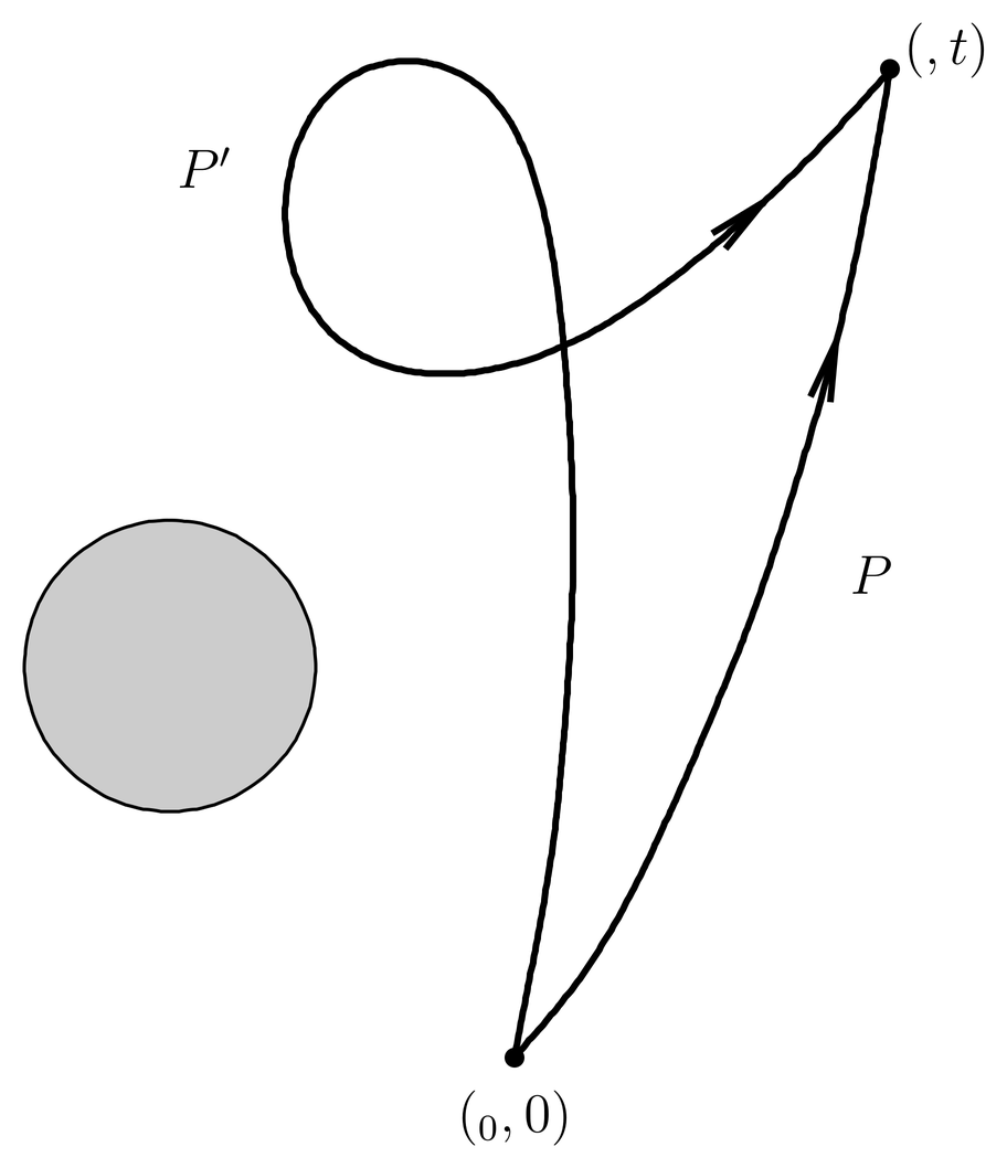
Figure 8:Any two paths that are homotopic, such as and , give rise to the same magnetic action.
But we prefer not to deal with Bessel functions so we shall examine the problem from the standpoint of the path integral rather than the energy eigenfunctions. This approach is not only more vivid in the physical picture it offers but is interesting in its own right.
The fields are time-independent so we write the propagator as
where we have used a version of (33) for the path integral. Here the path is denoted by for simplicity, and the notation stands for , including the constant factor seen in (33). It is understood that all paths satisfy the boundary conditions and , where , and are the parameters upon which depends, as illustrated in Figure 7. Also, we write the action functional as to avoid confusion with the vector potential . Since the Lagrangian of a particle in a magnetic field is
(see Magnetic Fields), the action functional is given explicitly by
which shows the decomposition of the action into a free part and a magnetic part. It is understood that the space of paths that we integrate over consists of all paths joining the initial and final space-time points and that do not enter the region , although they are allowed to loop or bounce off the walls of the solenoid as many times as they want. With this understanding, the free action alone would give us the propagator for the scattering of otherwise free particles from the hard walls of a cylinder at .
The magnetic action, however, modifies the propagator. Notice first that the factors cancel in the magnetic action, so that it does not depend on the parameterizatio of the path,
that is, it is just a line integral in 3-dimensional space. In fact, the magnetic action almost does not depend on the path at all, except for the endpoints. More precisely, consider two paths and that can be continuously deformed into one another without crossing the solenoid, as illustrated in Figure 8. Such paths are said to be homotopic. Then the magnetic actions along the two paths are identical,
since the difference as shown is the integral of around the closed loop obtained by first following and then following backwards to the initial point. This integral is the magnetic flux through the loop, which is zero since the magnetic field vanishes in the exterior region.
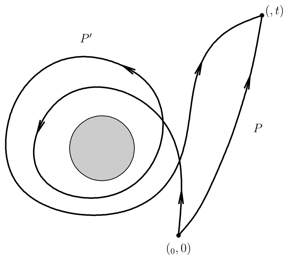
Figure 9:Two paths and that are not homotopic.
If the paths are not homotopic it is because they loop the solenoid a different number of times, as illustrated in Figure 9. In the figure, path loops the solenoid twice in the counterclockwise direction, relative to path . Thus, the difference in the magnetic actions is proportional to twice the flux through the solenoid,
where
To be more general let us choose a reference path and define . Then we define the winding number of any path as the number of times the closed loop goes around the solenoid in the counterclockwise direction, where means, first follow , then follow backwards. Then it is intuitively clear that any two paths are homotopic if and only if they have the same winding number. Also,
where is the winding number of path . Remember that in this discussion it is understood that all paths have the same endpoints and . This means that the space of paths can be broken up into homotopy classes, that is, a homotopy class indexed by is the set of all paths that have the same winding number. The integer takes on all values, positive, negative and zero. We denote the -th homotopy class by .
Then the path integration can be written,
As for the integrand, it can be written
Of the three factors shown, the middle one does not depend on at all, while the last depends only on the homotopy class. Thus, overall the path integral can be written
We see that the different homotopy classes contribute to the path integral with different overall phases, which are proportional to the winding number of the homotopy class. On the other hand, if there is no magnetic field in the solenoid, then the propagator is
a similar expression but without the extra phases attached to the homotopy classes. Thus, the homotopy classes interfere with each other in a different manner when there is a magnetic field in the solenoid.
Now notice that if the particle is an electron with then the extra phases can be written
where is the flux quantum (see The Flux Quantum). Thus if the magnetic flux in the solenoid is an integer multiple of a flux quantum then all these phase factors become unity, and the propagator becomes
which is the same as the propagator (72) in the absence of a magnetic field except for the overall factor . As for the latter, it can be eliminated by a gauge transformation. See Prob. Paragraph.
Altogether, we conclude that the magnetic field in the solenoid, where the particle never goes, influences both the energy eigenfunctions and the propagator of a charged particle in the exterior region.
Now we may return to the question, does the vector potential have effects in quantum mechanics that are not gauge-invariant, that is, effects that cannot be expressed purely in terms of ? The answer is no, since the extra phases that occur in the Aharonov-Bohm effect are expressed purely in terms of the flux in the solenoid, which is gauge invariant.
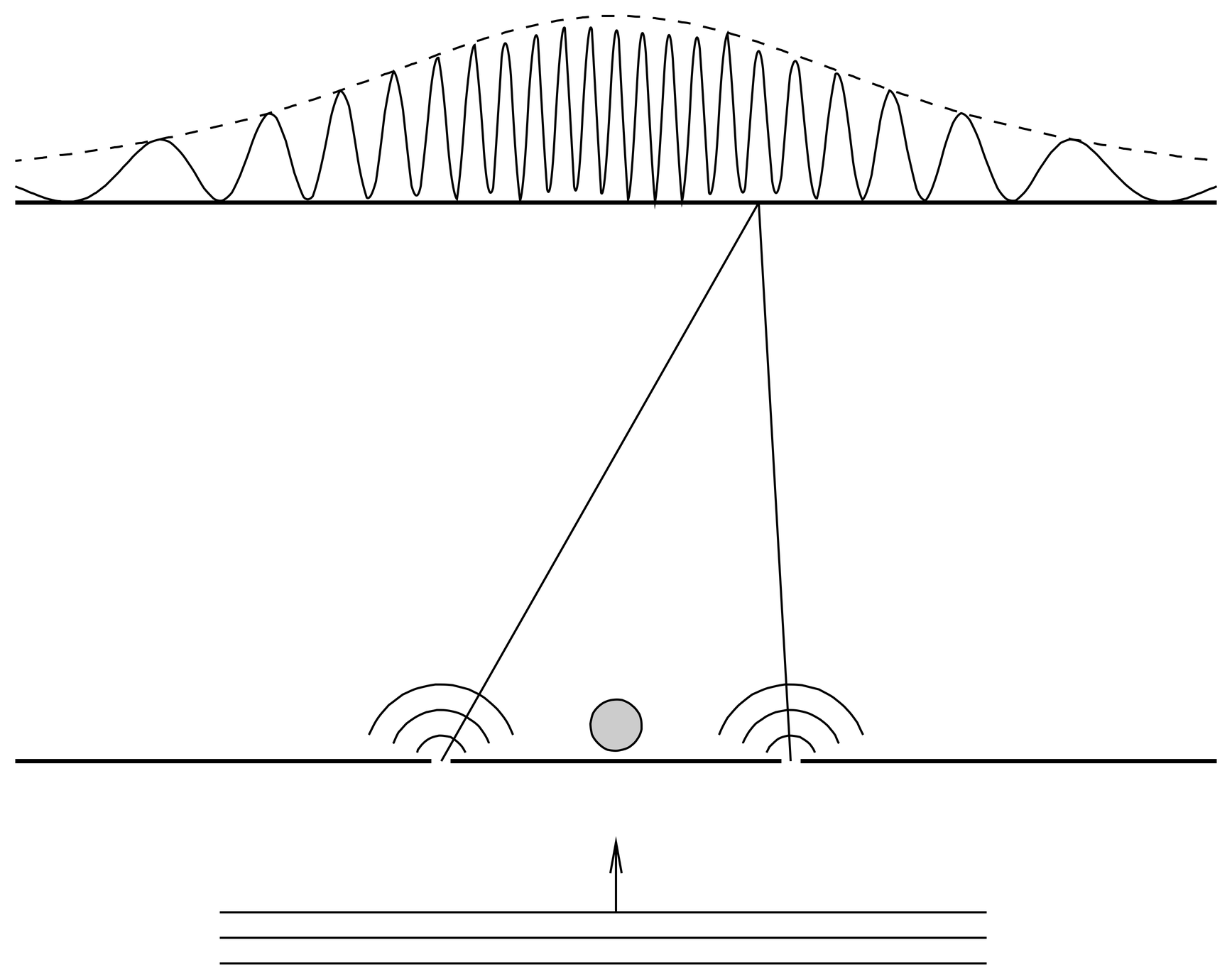
Figure 10:A solenoid carrying magnetic flux lies just behind the slitted screen of a double slit experiment. A plane wave of electrons is incident upon the slitted screen. The solenoid causes a phase relative shift of between the two paths joining the two slits to a point on the detection screen, where is a flux quantum.
So far we have merely shown that the energy eigenfunctions and the propagator in the exterior region depend on the flux in the solenoid. What difference does this make physically? One answer is given by an idealized double slit experiment, as illustrated in Figure 10. A plane wave is incident upon a screen with two slits, behind which an lies a solenoid carrying magnetic flux . The solenoid introduces a relative phase shift of between the two paths from the two slits to the detection screen. Thus, as the flux in the solenoid is changed, the interference pattern moves to the right or left under the envelope (the dotted line), returning to its original shape after has increased by an integer multiple of a flux quantum . Experiments along these lines have been carried out (see R. G. Chambers, Phys.\ Rev.\ Lett.\ 5, 3(1960)) with results that agree with the predictions of quantum mechanics.
Magnetic Monopoles
A magnetic monopole is a hypothetical particle that produces a magnetic field just like the Coulomb electric field of an ordinary charged particle. In spite of intensive searches, magnetic monopoles have never been observed. Nevertheless, they are much beloved by theorists, who find them interesting for many reasons. One is the argument first given by Dirac, which explains the quantization of electric charge, under the assumption that at least one magnetic monopole exists in the universe.
The quantization of electric charge refers to the fact that the charges of all known charged particles are integer multiples of the charge on the proton, what we denote by in this course (with ). In saying this we understand that we are talking about particles that can exist freely; otherwise, the quantum of charge is , carried by quarks. The accuracy to which this is known is very high. For example, if the positive charge on a proton and the negative charge on an electron did not exactly cancel one another, then a hydrogen atom would carry a net charge, a small one if the difference were small. This would mean that a hydrogen atom would accelerate in a uniform electric field. No such response is detected experimentally.
The quantization of charge is closely related to the conservation of charge. For example, a neutron decays into a proton, an electron, and an antineutrino. If the neutron and neutrino are genuinely neutral, and if the charge on the proton is not equal and opposite to the charge on the electron, then charge is not conserved in the reaction. It is known experimentally that the charge on the neutron is very close to zero.
Modern theoretical ideas about the quantization of charge relate it to the compactness of gauge groups, which in turn is related to ideas about extra (“compactified”) dimensions. While such ideas are very appealing, it cannot be said that they are well supported experimentally. In this we present the argument of Dirac for quantization of charge, based on magnetic monopoles.
We assume our monopole is infinitely massive and placed at the origin of the coordinates. The magnetic field has the form of a Coulomb field,
where is the strength of the monopole. This magnetic field satisfies
so the usual Maxwell equation is only valid for . Exactly at we have a -function singularity.
We will be interested in studying the quantum mechanics of a particle of charge in the field of the monopole (75). The Hamiltonian involves the vector potential , so we must find an such that of (75) can be written as . By writing out the curl in spherical coordinates (see Differential Operators in Spherical Coordinates), it is possible to uncurl and obtain . The answer is not unique, but one that readily suggests itself is
The vector potential is purely in the ~direction. Notice that while the magnetic field has full rotational symmetry, this vector potential has only rotational symmetry about the -axis.
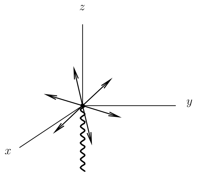
Figure 11:The vector potential is well behaved in the northern hemisphere, and has a singularity at the south pole (a string on the negative -axis).
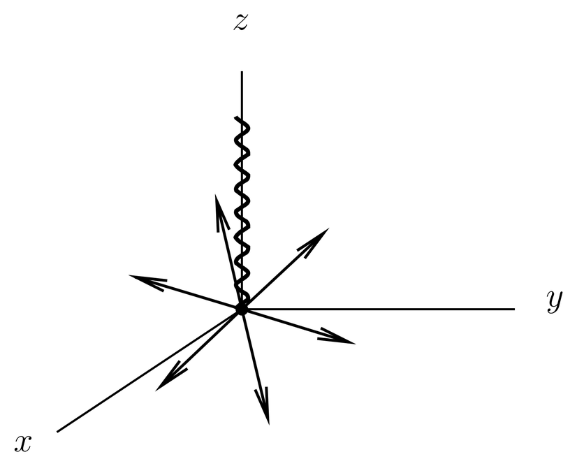
Figure 12:The vector potential is well behaved in the southern hemisphere, and has a singularity at the north pole (a string on the positive -axis).
The in the denominator of (77) suggests a singularity when or . Actually, there is no singularity at , because the factor goes to zero faster than as . But there is indeed a divergence as ; the magnitude of the vector potential diverges, and its direction becomes undefined (because is undefined when ). Thus there is a singularity of the vector potential on the negative -axis, which is called the string of the monopole. See Figure 11, where the string is indicated by the heavy wavy line. It is really a misnomer to call this the “string of the monopole”; the magnetic field itself is perfectly well behaved on the negative -axis. It would be better to call it the “string of the vector potential.”
Vector potentials are not unique, but can be changed by a gauge transformation. It is interesting to use a gauge scalar [see (86)] that is proportional to , the azimuthal angle. Note that
in spherical coordinates. For example, subtracting the gradient of from we obtain another vector potential (a different choice of gauge),
This vector potential is well behaved on the negative -axis but has a string on the positive -axis. See Figure 12.
We see that it is possible to move the string by performing a gauge transformation. Is it possible to get rid of the string altogether by a gauge transformation? That is, does there exist a vector potential for the magnetic field (75) that is regular everywhere (except of course at , where itself is singular)?
The answer is no, as can be proved by contradiction. Suppose there exists a vector potential that is regular everywhere except at , such that the monopole field (75) is given by . We imagine a small disk, really the end cap of a sphere, through which we wish to compute the magnetic flux, as in the first part of Figure 13. The flux is computed by
where the direction of integration around the boundary of the disk is shown by the arrow in the figure. Now we allow the disk to grow into the surface of a sphere, which gradually swallows the monopole. In the end the flux intercepted by the surface approaches , which can be computed by using (76) and Gauss’s law, while the circle around the boundary of the surface shrinks. As it does so, the integral (80) must approach zero, if is smooth as assumed, since the distance over which the integration takes place is going to zero. Thus we reach a contradiction, , and the assumption about the existence of a vector potential that is smooth everywhere in the region must be wrong. The vector potentials of magnetic monopoles inevitably have strings.
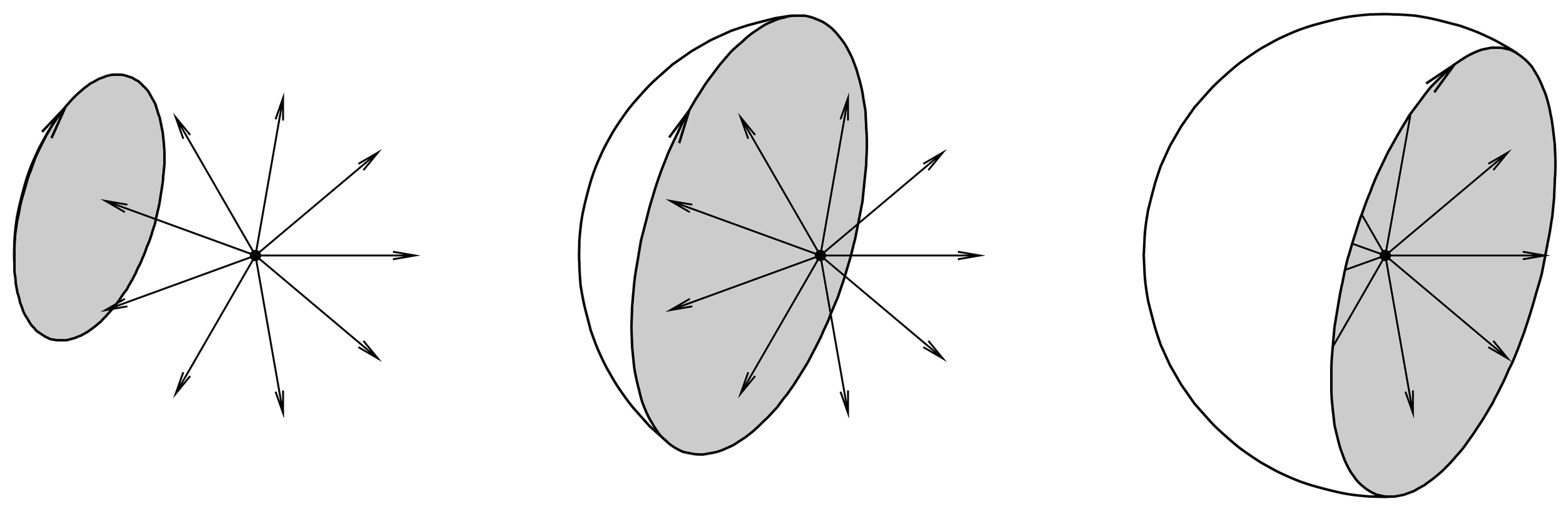
Figure 13:A surface swallowing a monopole. As it does so, the magnetic flux captured by the surface approaches , while the contour of integration around the boundary of the surface approaches zero (at the right of the figure).
If we examine the vector potentials and over a sphere centered on the monopole, we see that is regular (well behaved) over the northern hemisphere, and can be continued across the equator into the southern hemisphere, but not as far as the south pole. We call “north regular gauge.” As for , it is regular over the southern hemisphere and can be continued across the equator into the northern hemisphere, but not as far as the north pole. We call “south regular gauge.” Thus we can create two regions that overlap in a strip around the equator, with each vector potential regular in its own region. See Figure 14.
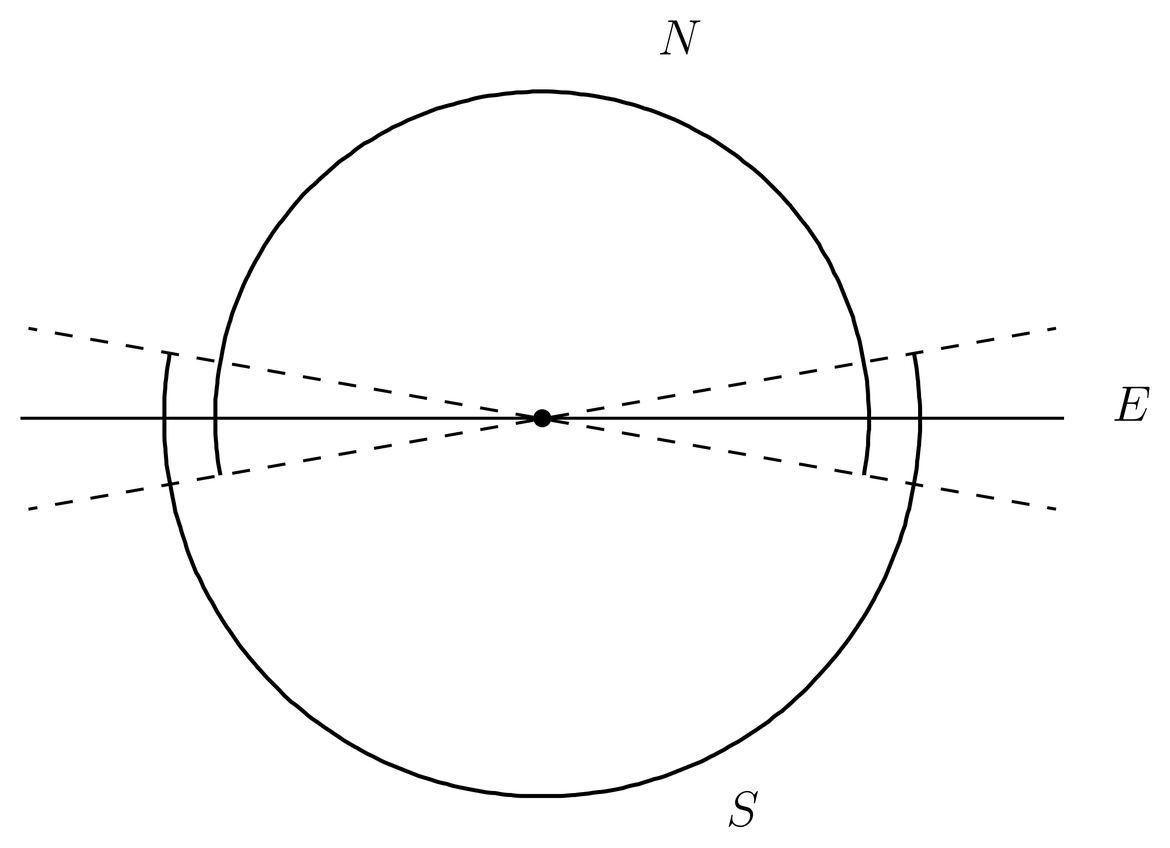
Figure 14:The regions , , of definition of and overlap at the equator .
To avoid singularities we must solve the Schr"odinger equation in patches. Suppose we do this, and find solutions and in the regions in which and are regular. In the overlap region, the solutions must be related by the gauge transformation. See (88), which in the present context becomes
where we have used for the gauge scalar. This equation applies around the equatorial strip.
The solution of the Schr"odinger equation must be continuous, otherwise the first derivative of would have a -function and the second derivative in the kinetic energy term would have a -function that could not be cancelled by any other term in the equation. But both and can be continuous in the overlap region only if the coefficient of the azimuthal angle in (81) is an integer, that is, if
But this implies
or the charge on the particle must be an integer multiple of a fundamental unit, proportional to the inverse of the charge on the monopole. Thus, if there exists even one monopole in the universe, the consistency of quantum mechanics requires the quantization of charge.
Dirac’s argument is fundamentally topological, and in modern theoretical treatments is expressed in terms of cohomology, fiber bundles and characteristic classes. Such topological concepts have assumed a prominent role in modern theoretical physics.
Problems
Problem 1.
Consider a spinless electron moving in the uniform magnetic field . Let be the quantum number of (the Landau level), and let be the eigenvalue of operator , as in Eq.~(\eqr\cn.13).
To find wave functions we need a third operator, in addition to } and and commuting with them, to form a complete set of commuting operators. The choice for the third operator was discussed above. That choice is useful for making the translational invariance in the -direction manifest. Here we make a different choice for the third operator, namely,
the angular momentum (or, rather, its -component), which makes the rotational invariance about the -axis manifest.
(84) is the usual definition of angular momentum, but it is only conserved if the vector potential is chosen to be rotationally invariant. Let us choose the gauge
If you plot the vector field in the - plane, or transform it to polar coordinates, you will see that it is invariant under rotations about the -axis.
Since , the kinetic momentum in the -direction is the same as the canonical momentum . Thus we will henceforth write instead of .
(a) Express in terms of variables and then in terms of . Show that it commutes with both and , so that all three operators, commute with one another. Let the eigenvalues of be written . Show that is an integer. For given , what are the allowed values of ?
Actually, a somewhat more convenient operator for the third member of the complete set is
another harmonic oscillator. Let be the usual harmonic oscillator quantum number for this oscillator. Express as a function of and . Henceforth let us take as the complete set of commuting observables.
(b) Now we work on finding the wave functions that are simultaneous eigenfunctions of . For the rest of this problem, let us choose units so that , which simplifies the algebra and which entails no loss of physics since physical units can always be restored in the final formulas.
First show that an eigenfunction of with eigenvalue has the form
This is the easy operator.
Choosing so that the function is also an eigenfunction of both and takes more work. We first work on the double ground state , . Introduce annihilation and creation operators , for oscillator and another pair , for oscillator . The double ground state wave function must be annihilated by both and . That is, we want
Write out and as differential operators in and .
The subsequent analysis is simplified if we use complex coordinates , in the - plane, defined by
so that
Transform the differential operators for and to the , coordinates, and solve (88) for . Normalize it.
(c) Now write out differential operators in the , coordinates for the creation operators and . Use them to obtain the normalized wave function for , .
(d) Use the Rodriguez formula for the associated Laguerre polynomials,
[see Abramowitz and Stegun, Eq.~(22.11.6)], to express the normalized wavefunction for any values of and in terms of associated Laguerre polynomials. Hint: Use the identity,
where is any function.
Problem 2.
Consider the motion of an electron of charge in the field of a magnetic monopole. Assume the monopole is infinitely massive in comparison to the electron. The monopole produces a field,
where is a constant. Although monopoles have never been observed, nevertheless people have carried out experiments to search for them. In such experiments, it is important to know the behavior of ordinary matter in a monopole field, in order to recognize the signatures a monopole would make in experimental apparatus.
(a) Write down Newton’s laws for the electron motion. You may use the abbreviation,
To solve these equations of motion, we begin by a search for constants of motion. If it were an electric monopole instead of a magnetic monopole, then we would obviously have four constants of motion: the energy and angular momentum . Show that the usual (orbital) angular momentum vector is not conserved. Show that is conserved, however. This gives you two time-independent constants of motion, , which are not enough to obtain the complete solution. Therefore we must find more constants of motion.
(b) Consider the vector potential,
This vector potential is well behaved everywhere except on the -axis (both positive and negative). Verify that this vector potential gives the magnetic field of (93). This vector potential is invariant under rotations about the -axis, that is, the angle is ignorable. Use this vector potential in a classical Lagrangian in spherical coordinates, and use Noether’s theorem to obtain another conserved quantity (in addition to , ). (Noether’s theorem says that if a Lagrangian is independent of , the is conserved.) Show that this quantity is plus another quantity which you may call . Write , so that is the new conserved quantity. As the notation suggests, interpret as the -component of a vector , i.e., guess the formula for (all 3 components). Hint: to help you with the guess, transform to rectangular coordinates. By resorting to Newton’s laws, show explicitly that is conserved. You now have four time-independent constants of motion, . There are only four, because is a function of ; show this.
(c) By playing around with dot products of various vectors and looking for exact time derivatives, find more constants of motion. Use these to find as a function of . Show that the electron can reach the singularity at only if .
(d) Show that the orbit lies on a cone whose apex is at the origin. Find the opening angle of the cone as a function of . Find a vector which specifies the axis of the cone. Assume , and let occur at the point of closest approach. Find the distance of closest approach as a function of .
(e) Choose the axes so that is parallel to the -axis. Find as functions of .
(f) The solution of this problem was first carried out by H.~Poincar'e, Compt.\ Rend.\ 123, 530(1896). Poincar'e pointed out that the orbit is a geodesic on the cone, since the force is always orthogonal to the cone. This follows since the tangent plane to the cone is spanned by the velocity vector and the radius vector , and for the monopole field the magnetic force is orthogonal to both. But a cone is a flat surface, as shown by the fact that it can be unrolled into a plane.
Take a piece of plain white paper, and draw a straight line on it. This line is a geodesic. Now roll the paper into a cone. Try cones of different opening angles and different relations to the straight line. The straight line now appears as the orbit of an electron in the field of a monopole. You can see how it spirals in on the cone, reaching a point of closest approach, and then sprirals out.
Problem 3.
This problem is relevant for the quantum Hall effect. Consider the motion of a spinless particle of charge in the magnetic field and electric field , where and are positive constants (the fields are uniform). In this problem we ignore the motion in the -direction, and just work with a 2-dimensional problem in the - plane.
To simplify the algebra, choose units so that , and let and (here is not necessarily small). Notice that is the frequency of the circular motion in the absence of an electric field.
The classical motion is along a circle that “drifts” in the -direction with velocity,
At a certain point in the calculation you may find this a convenient substitution.
(a) Express the Hamiltonian as a function of the operators . In the case of the uniform magnetic field (without ) we found that commuted with any function of or . What functions of and does commute with now that we have an electric field? What is the energy of a state that is an eigenstate of both and ? Express the energy in terms of some reasonable quantum number(s).
(b) Choose a gauge , where is the unit vector in the -direction. Let . Find the most general wave function that satisfies this equation.
(c) Now let , where is the energy, and where has the form determined in part (b). Express the solution in terms of , defined to be the normalized harmonic oscillator eigenfunction for quantum number .
(d) Compute the -component of the probability flux, properly interpreted as a particle flux since the wave function is not normalizable. Integrate this flux over the line to get the number of particles/unit time crossing this line. Notice the relation to the drift velocity.
Problem 4.
This problem has some things in common with Prob.~Paragraph, but the notation is independent of that of that problem.
(a) Consider an electron moving in the magnetic field . We ignore the spin of the electron (we treat it as if it were a spinless particle), and we ignore the motion in the -direction. Thus, we have a 2-dimensional problem, in the - plane.
In this problem I recommend that you use units such that , where is the gyrofrequency [see (12)]. Also, use the vector potential,
As in the notes above I recommend that you put hats on the symbols , , , , , , and when operators are intended, and omit the hats when -numbers or classical values are intended. For other operators this distinction will not be necessary and you can omit the hats.
The classical guiding center is defined by
which are dimensionless versions of (18). Also define the operators , , and by
and
It helps to notice that and are like ’s, while and are like ’s [see (24)].
Let be the wave function such that
Find the normalized wave function . Hint: I suggest you work with and . We will denote the ket corresponding to the wave function by .
We will take the complete set of commuting observables for this problem to be , where is the Hamiltonian and
With this understanding, explain the meaning of the 00-subscript on .
(b) Define operators,
Explain why and commute with one another.
Letting be an arbitrary wave function, work out
It helps to notice that both and can be factored into commuting operators, each of which is either a pure configuration space displacement, or one in momentum space. If you use this fact, explain why the factors commute.
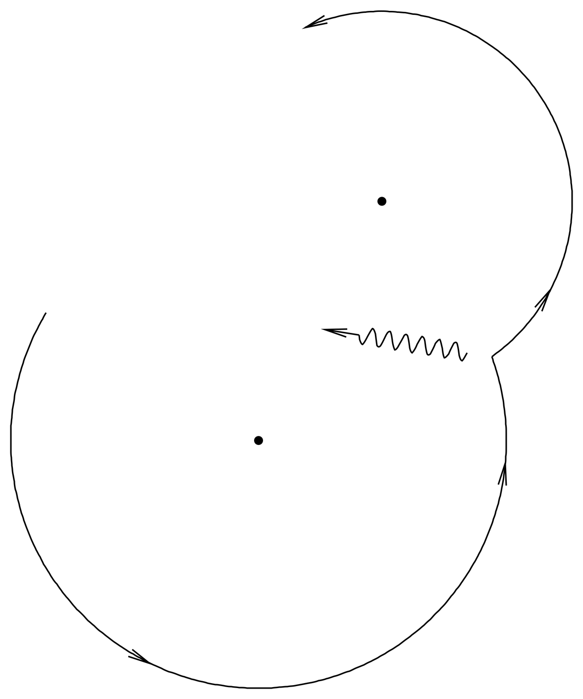
Figure 15:When the electron emits a photon the recoil causes both the velocity and guiding center position to change. The actual position does not.
(c) If the initial conditions for the classical motion are , , find the classical solutions , .
(d) Let be a solution of the time-dependent Schr"odinger equation. We are interested in the solution for which the initial condition is the wave function corresponding to the state
with and . That is,
Find .
Hint: you may find the following definitions convenient:
and
Finally, at some point you may wish to write
where and were determined in part~(c).
(e) Suppose the electron is in the state at times . It emits a photon at whose momentum is in the negative -direction, causing the expectation value of the velocity of the electron, just after the photon is emitted, to be . Find the probability that for the electron is in Landau level . Express your answer in ordinary (not dimensionless) units. If you have done Prob. Paragraph, compare your answer to the answer of that problem.
Hints: Note that the impulse delivered by the photon changes both the velocity and the guiding center position, as is necessary for consistency with (98) since the particle position does not change. This is also obvious from a picture (see Figure 15). Thus, the state of the system just after the photon is emitted is not the same as the initial condition in part~(d).