05. Time Evolution in Quantum Mechanics
Introduction
In these notes we develop the formalism of time evolution in quantum mechanics, continuing the quasi-axiomatic approach that we have been following in earlier notes. First we introduce the time evolution operator and define the Hamiltonian in terms of it. Then we discuss the evolution of state vectors and the Schr"odinger equation, the evolution of observables in the Heisenberg picture and the Heisenberg equations of motion, the evolution of the density operator, and the initial value problem. Next we introduce the Hamiltonian for potential motion and discuss aspects of it, including wave function representations of the Schr"odinger equation, the probability density and current, and the Ehrenfest relations. Finally we discuss the Schr"odinger equation for a charged particle in a magnetic field, and discuss its transformation properties under gauge transformations.
The Time-Evolution Operator
Let the pure state of a system at some initial time be described by the state vector , and let the state at some final time be described by . We postulate that these two state vectors are related by a linear operator , parameterized by the two times, that is,
We write the final time first and the initial time second in . This is another (the seventh) postulate of quantum mechanics, which we can add to the list in The Postulates of Quantum Mechanics (Revised).
The operator must satisfy the following three properties. First, it reduces to the identity at ,
Second, it must be unitary in order to preserve probabilities,
For example, the probability of finding a particle somewhere in space must be 1, and, assuming particles are neither created or destroyed, this probability must be independent of time. In relativistic interactions particles are created and destroyed, but even here we require the unitarity of . The logic is that if we measure some observable, the probability of getting some answer must be 1, independent of . As for measuring the position of a particle in relativity theory, we will see later in the course that the position operator is not well defined in relativistic quantum mechanics, precisely because of the possibility of particle creation or destruction.
The third property says that if we evolve a system from some initial time to some intermediate time , and then from to some final time , we must get the same answer as evolving directly from to . In other words, we can regard the state at any intermediate time as the initial conditions for the second half of the time evolution. According to this composition property,
The Hamiltonian
Now consider an infinitesimal time evolution from time to , where is small. We expand out to first order in and write the correction term as follows:
where the ellipsis indicates higher order terms in . Effectively, we have defined the operator as
We introduce the factor of in (6) in order to make Hermitian. This follows from the unitarity of , precisely as in the demonstration of the Hermiticity of in The Generator of Translations. The operator depends on in general because the right-hand side of (6) does so.
The operator can be regarded as the generator of time translations in quantum mechanics, because it gives the small correction needed to advance a state from time to . Evolution over a finite time interval can be regarded as the result of a large number of small displacements in time, so knowing in principle allows us to evolve the system over any time interval. Since it is Hermitian, presumably corresponds to something we can observe.
The classical Hamiltonian is considered the generator of time translations in classical mechanics. This means that for small time increments we can calculate the correction in or or any other classical observable by forming the Poisson bracket with . To see this explicitly, let be a classical observable (for a particle moving in one dimension, for simplicity), which acquires a time dependence because and evolve in time as a particle moves along its orbit. Then, working to first order in a small time increment , we have
where we use Hamilton’s equations, (78), and the definition of the Poisson bracket, (100). This should be compared to (69), which shows the analogous role of the momentum in classical mechanics as the generator of translations.
Because of the role of the classical Hamiltonian as the generator of time translations, we guess that is closely related to the operator that we should define as the quantum Hamiltonian, denoted by (with a hat to distinguish it from the classical Hamiltonian ). We cannot have because has units of inverse time, while has units of energy. We fix this by defining
With this definition, the infinitesimal time evolution (5) becomes
We remark that Hamiltonians in classical mechanics depend on time when there are time-dependent forces or fields present. See the discussion in Conservation of Energy. For example, the motion of a charged particle in an electromagnetic wave is described by a time-dependent Hamiltonian. We expect the same to be true in quantum mechanics, so depends on , in general. As in classical mechanics, however, time-independent Hamiltonians are an important special case, and offer some simplifications.
Our presentation leads to the question of whether the in (8) is the same as in (70), . See The Momentum in Quantum Mechanics: The History for an overview of the history of the relations and . Here we simply note that these relations are obviously the space- and time-components of a single 4-vector, in which energy and momentum are generators of displacements in time and space, respectively. Relativistic covariance requires that the ’s in these relations be the same. We are only concerning ourselves with the nonrelativistic theory at this point, but it is obvious that relativistic covariance will be impossible to establish if these ’s are different.
Differential Equations for Time Evolution
To obtain a differential equation for we take the derivative with respect to the final time , using the definition of the derivative:
But by the composition property (4), we can write
so the operator can be factored out to the right in (10), giving
The remaining limit is , which by (6) and (8) is . Altogether, (12) becomes
This differential equation is subject to the initial conditions (2). In practice is usually a given operator as a function of time and we wish to solve for . With the given initial conditions, the solution is unique.
Now differentiating (1) with respect to and using (13), we obtain a differential equation for the state vector ,
which is subject to the given initial condition for the state vector. This is the Schr"odinger equation. This is a ket equation that differs only trivially from the operator equation (13).
The case that the Hamiltonian is independent of time, , is important in practice. In this case, (13) has the solution,
showing that only depends on the elapsed time when is independent of . Writing simply for the elapsed time (or choosing ), we have
In this case, commutes with .
In the general case in which depends on time, there is no simple solution for . In this case does not commute with , nor for that matter does it usually commute with itself at different times.
The Heisenberg Picture
The time evolution of a classical observable along an orbit is given by (98) or (101). In quantum mechanics we see a closer analogy with classical mechanics if we allow observables to evolve in time. Up to this point in our discussion of time evolution in quantum mechanics we have used the Schr"odinger picture, in which kets evolve according to the Schr"odinger equation (14), and operators do not evolve (unless they have an explicit time dependence, in which case their only evolution is due to this time dependence). We shall continue to use the Schr"odinger picture for most of this course, but there are certain problems and topics that are best handled in the Heisenberg picture, in which kets do not evolve in time but operators do. We shall now explain these two pictures and the relation between them.
In the following we drop the hats on , it being understood that we are speaking of the quantum Hamiltonian.
The Schr"odinger and Heisenberg pictures differ by a time-dependent, unitary transformation. In the following we shall put an subscript on kets and operators in the Schr"odinger picture and an subscript on them in the Heisenberg picture. If a ket or an operator appears without a subscript, the Schr"odinger picture is assumed. If is the time-dependent state vector in the Schr"odinger picture, then the state vector in the Heisenberg picture is defined by
By (1) and (3), this is equivalent to
where is the initial time. The state vector in the Heisenberg picture does not evolve because it is equal to the ket in the Schr"odinger picture at the initial time . As for operators, if is an operator in the Schr"odinger picture, which for generality we allow to have an explicit time dependence, then the corresponding operator in the Heisenberg picture is
The Heisenberg operator has a time dependence for two reasons, first because the Schr"odinger operator may have an (explicit) time dependence, and second because the operators and depend on time, what we regard as the implicit time dependence. Notice that the Heisenberg operator depends on time even if the Schr"odinger operator does not (because of the implicit time dependence). See Conservation of Energy for a discussion of explicit and implicit time dependence in classical observables.
There is no evolution equation for in the Heisenberg picture, but the operators obey an evolution equation obtained by taking the derivative of the definition (19) and using (13). This gives
where is the Hamiltonian in the Schr"odinger picture, which may be time dependent. But by inserting the product between and in the first two terms above, the result can be written purely in terms of operators in the Heisenberg picture,
where the last term means, differentiate with respect to its explicit time dependence in the Schr"odinger picture, then convert to the Heisenberg picture. This may also be written
whereupon the analogy with the classical equation (101) is more striking. Equations~(21) or (22) are the Heisenberg equations of motion for operators.
Algebraic Relations Same in Both Pictures
Suppose we have an operator in the Schr"odinger picture, so that in the Heisenberg picture it is , where . Then if for some function , it turns out that
This is easy to see in the case that is a polynomial or power series, for example, if we have
but the result can be proved more generally by using the definition of a function of an operator given in A Function of an Observable. Likewise, suppose we have an algebraic relation in the Schr"odinger picture such as , where and need not commute. Then it is easy to show that . In other words, algebraic relations among operators in the Schr"odinger picture are converted into the corresponding algebraic relations in the Heisenberg picture simply by replacing the subscripts with ’s.
In particular, commutation relations have the same form in both pictures. If , then . Also, if is a potential energy in the Schr"odinger picture, then
is the potential energy in the Heisenberg picture. This means that the Hamiltonian has the same form in both pictures, for example, if
then
The Heisenberg and Schr"odinger Pictures are Physically Equivalent
All measurable quantities in quantum mechanics can be expressed in terms of matrix elements of the form . These, however, are the same in both the Heisenberg and Schr"odinger pictures,
since the unitary operators cancel when (17) and (19) are substituted. Thus, if we can find the time evolution of operators in the Heisenberg picture, we can predict the outcome of all experiments equally well as by finding the time evolution of the state vector in the Schr"odinger picture. For some problems, the Heisenberg picture is easier to use (the harmonic oscillator, for example). In addition, the Heisenberg picture is needed in relativistic quantum field theory to establish manifest Lorentz covariance. Although most of nonrelativistic quantum mechanics is usually carried out in the Schr"odinger picture (and also in this course), it can be argued that the Heisenberg picture is more fundamental.
In the special case that the Schr"odinger Hamiltonian is independent of time, the operator is a function of and so commutes with it, according to (16). Thus, in this case, the Schr"odinger and Heisenberg Hamiltonians are the same,
where we have set as in (16).
There are other pictures besides the Schr"odinger and Heisenberg pictures. In the interaction picture, which we will take up in 34. Time-Dependent Perturbation Theory, the time dependence due to some unperturbed Hamiltonian is stripped off from the kets and transferred to the operators. But the time dependence remaining from some perturbation is left on the kets. Thus, the interaction picture is intermediate between the Schr"odinger and Heisenberg pictures. It is especially useful in time-dependent perturbation theory and scattering theory.
Time Evolution of the Density Operator
(14), the Schr"odinger equation, gives the time evolution of the state vector in quantum mechanics. As we have seen in 03. The Density Operator, however, the state of a quantum system is described in general by a density operator, not a state vector. Therefore we require an equation of evolution for the density operator. We work here in the Schr"odinger picture, and consider the density operator for a discrete ensemble of pure states with statistical weights , as in (16). The density operator is a function of time because the states are functions of time. We put a hat on to distinguish it from the classical density discussed in Classical Statistical Mechanics.
At the initial time the density operator is given by
while at the final time it is
Differentiating this last expression with respect to time and using (13), we find
This equation replaces the Schr"odinger equation when we have mixed states. By a slight change (32) can be written
whereupon the analogy with the classical Liouville equation (112) is more clear. (32) looks similar to the Heisenberg equation of motion for some observable, (22), but they are not the same since we are working here in the Schr"odinger picture.
Commutators and Poisson Brackets
Comparing the quantum equations (22) and (33) with their classical counterparts (101) and (112), respectively, we see that one goes into the other if we map commutators into Poisson brackets according to the rule,
This association was first noticed by Dirac, and it helped him to establish the formal structure of quantum mechanics on the classical model. In important cases it is an exact correspondence, that is, quantum commutators are the same as classical Poisson brackets, apart from the factor and a reinterpretation of the symbols as operators (quantum observables) instead of classical observables. Compare, for example, the classical canonical Poisson bracket relations (108) with the Heisenberg-Born commutation relations (74). Another example is the classical Poisson bracket relations for the components of orbital angular momentum, ,
which may be compared to the quantum commutation relations for the components of the angular momentum operator,
In other cases, Dirac’s correspondence (34) is only approximate.
Constants of Motion
In classical mechanics, an observable is a constant of motion if its value is constant as and evolve along an orbit. For simplicity in this we only speak of observables without an explicit time dependence, and we assume that the Hamiltonian, too, has no explicit time dependence. But according to (101), this means that has vanishing Poisson bracket with the Hamiltonian, .
Similarly, in quantum mechanics, we say that an observable without an explicit time dependence is a constant of motion if it commutes with the Hamiltonian, . Then the Heisenberg equations of motion (21) imply
This in turn implies that the expectation value of with respect to any state is constant in time,
where, as we have seen, the expectation value can be computed in either picture (Schr"odinger or Heisenberg).
Energy eigenstates in many practical problems are expressed as simultaneous eigenstates of a complete set of commuting observables, of which the Hamiltonian is one. For example, in central force motion we often use . But since the other observables in the list, besides the Hamiltonian, all commute with the Hamiltonian, they are all constants of motion, and their expectation values with respect to arbitrary states are independent of time. And since the Hamiltonian commutes with itself, it is also a constant of motion.
The Initial Value Problem for Time-Independent Hamiltonians
The initial value problem refers to the problem of finding the final state at some time , given the initial state at some initial time . When the Hamiltonian is time-independent, it is possible to give an explicit solution to the initial value problem in terms of the eigenstates and eigenvalues of the Hamiltonian.
Suppose in (14) is time-independent. Let us denote its eigenstates by and corresponding eigenvalues by , so that
where can stand for one or more quantum numbers needed to specify an energy eigenstate. For simplicity we assume the index is discrete, but the formulas are easily extended to handle a continuous or mixed spectrum. Let us expand the time-dependent state in terms of the energy eigenstates,
where the expansion coefficients depend on time. Then by substituting (40) into (14), we find
or,
Thus we have
where
These results are equivalent to expanding the time-evolution operator in energy eigenstates,
This is a special case of a function of an observable expressed in terms of the projectors of that observable, as described in A Function of an Observable.
Often the easiest way to solve the initial value problem in quantum mechanics is first to find the eigenfunctions of the Hamiltonian, then to compute the expansion coefficients of at by (44), and finally to sum the series (43). This only works for time-independent Hamiltonians, however.
In particular, if the system is known to be in an energy eigenstate at , then it stays in this state forever. The only thing that changes in time is the overall phase of the state, . For this reason an energy eigenstate is also called a stationary state.
Hamiltonian for Potential Motion
So far we have defined the Hamiltonian operator as the generator of time evolution, but we have not said what the Hamiltonian actually is in any specific case. The simplest case is that of a particle of mass moving in a potential , which for generality we allow to depend on time. See The Lagrangian, and the Case for the physical meaning of time-dependent potentials, including an example. See also See. Conservation of Energy for a discussion of time-dependent Hamiltonians. In practice, the potential is often time-independent. The classical equations of motion are
where . The classical Hamiltonian is a single-particle version of (83),
To obtain the quantum Hamiltonian, we take this formula and reinterpret the classical observables and as operators acting on the ket space spanned by the position eigenkets , as in 04. Spatial Degrees of Freedom. This space is isomorphic to the space of wave functions . The operators and satisfy the Heisenberg-Born commutation relations (74). As in classical mechanics, the Hamiltonian (47) is the sum of the kinetic and the potential energies.
Quantum mechanics must go over to classical mechanics in the limit in which is small, that is, when all actions of a problem are large in comparison to . So it is an educated guess that we can adopt a classical Hamiltonian in this manner, reinterpret it, and get the correct quantum Hamiltonian. Ultimately, the success of our guess must be verified by comparison with experiment, or comparison with a more fundamental theory that we trust. And of course we trust fundamental theories when they have been verified by experiment. There is no process of logical deduction to obtain quantum mechanics from classical mechanics, since new physics is involved.
The potentials that are used in practice are often phenomenological models that represent guesses or hopes that some complicated physics can be represented by a potential. For example, we may try to represent the interaction of two atoms, or of a proton and a neutron, by a potential. Actually, atoms and nucleons are composite particles with internal structure, and their interactions can only be represented by a potential in an approximate manner.
A large part of atomic, molecular and condensed matter physics can be understood in terms of the electrostatic interactions of charged particles. These are described by the potential (24), which can be regarded as “fundamental.” But effects involving spin, magnetic fields, relativistic corrections, the emission and absorption of radiation and other phenomena require other types of Hamiltonians. We will consider magnetic fields below in Particles in Electromagnetic Fields, and the other generalizations will be taken up later in the course.
The multiparticle generalization of (47) is straightforward. Let there be particles with masses , positions and momenta , and assume that they interact by means of a potential. Then the classical Hamiltonian is
In a multiparticle system, the wave function is . It is a function defined over the multidimensional configuration space (see \classmech.3).
Representations of the Schr"odinger Equation
The Hamiltonian (47) is presented in terms of operators and . We will not put hats on these operators as we did in 04. Spatial Degrees of Freedom, since it will usually be clear from context whether a quantum operator is intended and or a -number. These operators are represented in different ways in different representations, as discussed in Secs. Properties of the Momentum and The Momentum Representation (see Table 1). We now translate the ket version of the Schr"odinger equation, (14), into its configuration space representation, using the Hamiltonian (47). We write . Then using (20) and (78) or Table 1 for the actions of and on configuration space wave functions, we obtain
If the potential is independent of time, then we often wish to find the energy eigenfunctions of the Hamiltonian, call them where are the energy eigenkets as in (39). These satisfy
which is the configuration space representation of (39). Equations (49) and (50) are the time-dependent and time-independent versions, respectively, of the Schr"odinger equation in configuration space, for a single particle moving in a given potential.
We can also write down the Schr"odinger equation in momentum space. In the time-independent version, it is
where and where
The first term on the left of (51) (the kinetic energy) is a multiplicative operator in momentum space, which is simpler than the differential operator (the Laplacian) that occurs in configuration space. The potential, on the other hand, has become an integral operator. The momentum space version of the Schr"odinger equation is useful for some problems, notably the hydrogen atom.
The Probability Density and Current
Let us consider a single particle moving in three-dimensional space under the influence of a potential , as described by the Hamiltonian (40). The potential may be time-dependent. Let us write
for the probability density on configuration space (not to be confused with the density operator). The probability density changes in time, in general, but the integral over all space,
does not, since it is just the square norm of the wave function which is constant in time due to the unitarity of .
Associated with the probability density is a probability current satisfying
The current is conveniently expressed in terms of the velocity operator, which in the configuration representation is given by
The current itself is
The current looks like the real part of the expectation value of , but it is not since we do not integrate over all space. It is however the real part of the integrand of that expectation value. It is straightforward to prove the continuity equation (55) with the aid of the Schr"odinger equation (49).
Notice that if is an energy eigenfunction , then is independent of time and the continuity equation reduces to . Also, if the Hamiltonian is of the kinetic-plus-potential form, then time-reversal invariance (see 06. Topics in One-Dimensional Wave Mechanics{} and \timerev) implies that the energy eigenfunctions can be chosen to be real. In that case, .
The definition of the probability current depends on the system. For the case considered here, a single particle moving in 3-dimensional space, the probability current is a 3-vector. In an -particle system the probability current is a -vector on the -dimensional configuration space. Also, even for a single particle, the definition is modified in the presence of magnetic fields, as we shall explain in Particles in Electromagnetic Fields below, or when there is spin.
Physical Significance of the Probability Density and Current
The existence of a probability density and current that satisfy the continuity equation (55) is usually regarded as an essential part of the probabilistic interpretation of the wave function . There is, however, the question of the physical interpretation of and .
The physical interpretation of the density is clear on the basis of the postulates of quantum mechanics: It gives the distribution of measured positions of the particle when measurements are made across an ensemble of identically prepared systems. We should not think that the particle in an individual system has been somehow smeared around in space. If we make a measurement of the position of the particle, we find some definite value, not some fraction of a particle in one region and another fraction in another. In particular, if the particle has charge, we never measure a fraction of the charge. Thus, fundamentally, the density describes the statistics of the ensemble, not some kind of smearing of an individual system. Nevertheless, there are circumstances in which the latter interpretation also appears, as we shall explain. Similar considerations apply to the current .
In the case of a charged particle, it is suggestive to multiply both the probability density and current by the charge of the particle , and to write
since then the continuity equation for and looks like the law of conservation of charge,
But now the question arises, do this and serve as sources for electromagnetic fields? If so, are these fields measurable? That is, are electric and magnetic fields produced by the average positions and motions of the charged particle across the ensemble, or by their “actual” positions and velocities in an individual system? (We put “actual” in quotes because position and velocity do not commute, and so cannot simultaneously have a precise value.)
Consider, for example, a hydrogen atom in the ground state. The wave function for the electron is rotationally symmetric and dies off exponentially with a scale length which is the Bohr radius, so the probability density and effective charge density do the same. At a distance large compared to the Bohr radius, the electron wave function and hence probability density are essentially zero. Since the probability density is rotationally symmetric, that is, it is a function only of the radius , the electric field produced by is easy to calculate by Gauss’s law. The electric field is purely in the radial direction, and, far from the proton, it is the same as that of an electron at the origin (the position of the proton). If we add the electric field of the proton, the total electric field far from the hydrogen atom is zero.
On the other hand, in a classical model of the hydrogen atom, in which the electron has a definite position, the electric field produced by the electron and proton is a dipole field, which falls off as . Moreover, the dipole is time-dependent, as the electron moves around in its orbit. This is quite different from the electric field produced by the average charge density .
If we take an actual hydrogen atom in the ground state and measure the electric field, which do we get? A dipole field, or a field that falls off exponentially to zero within a short distance?
This is a somewhat subtle question. In the first place, the electron is in orbit around the proton, so if we wish to see a dipole field we would need to make the measurement on a time scale shorter than the orbital period of the electron, which is something like 10-16 seconds. It would be hard to make such a measurement in practice. On longer time scales we will see an average field. In fact, taking an expectation value of an observable with respect to an energy eigenfunction is similar to making a time average in classical mechanics. (The one goes over into the other in the classical limit.) This can be seen crudely by the time-energy uncertainty principle, . In an energy eigenstate, since the energy is exactly known. Thus the time is completely unknown.
But if it were practical to make a measurement of the electric field on a very short time scale, what would we find? To answer this question, we must first remember that according to the measurement postulates of quantum mechanics, all observables are represented by operators that act on some ket space. This must also apply to the measurement of the electric field that we are contemplating. According to classical electromagnetic theory, the electric field at field point due to an electron of charge at position is
in the electrostatic approximation. There are two measurable quantities that appear in this formula, the position of the electron and the value of the electric field at observation point . But the observation point is not an observable, since we are not measuring it; it is just the place where we make the measurement of . With this understanding, we see that is a function of , that is, is an operator (really, a vector of operators) that act on the ket space for the electron. Since the components of commute with one another, so also do the components of , and at one point commutes with at another point . In fact, by measuring at any point and knowing the charge of the electron, we can solve (60) for , the position of the electron. Measuring the electric field at a point is thus equivalent to measuring the position of the electron. The value measured in any individual system is thus a dipole field, as in the classical case.
We emphasize that this discussion is based on the electrostatic approximation, in which we ignore the retardation in the communication between the source of the field (the electron, at position ) and the observer (at position ). We also ignore magnetic fields and other effects that lie outside the electrostatic approximation.
It is possible to make a variation on this situation that is not hampered by short time scales. Consider a double slit (really, a double hole) experiment, in which a plane wave (a pure state of a given energy) of electrons is directed against a screen . See Figure 1. There are two holes in the screen that are large compared to the wavelength, so that two parallel beams emerge on the other side. We assume the beams are wide enough to ignore diffraction effects (the spreading of the beam) over the extent of the experiment. Then probability density is nonzero inside two cylinders (the two beams) downstream from the holes. This is a variation in the double slit experiment, in which one of the questions is whether a single electron passes somehow through both holes, or how we can know which hole it passed through.
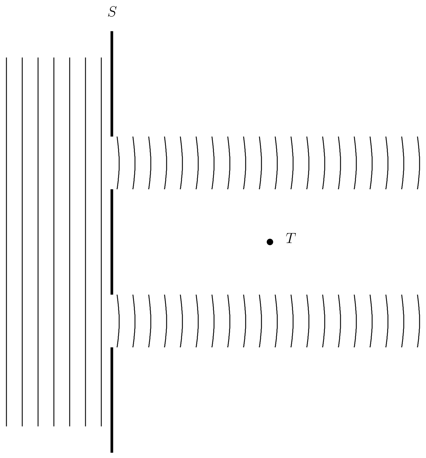
Figure 1:A variation of the double slit experiment, in which we attempt to measure which hole in the screen the electron passed through by measuring the electric field produced on test charge as the electron passes by.
Let us place a test charge half way between the two beams, as in the figure. By symmetry, the electric field produced by is zero on the axis between the two beams, so if is affected by the electric field of the particle smeared out according to , then it should not move. But if we think of an individual system in a classical sense, each electron will pass by the test charge on one side or the other. If we imagine that is massive enough that it does not move much while the electron is passing by, then the main effect of the electron is to deliver an impulse in the transverse direction (up or down in the figure). If we see which direction the test charge moves, we can detect which of the two beams the electron was in. So now the question is, what does the test particle really do in a double hole experiment of this type? Does it respond to the average electric field, or to the field of an individual electron, as in a classical model?
To answer this question we must realize that the test particle is a quantum mechanical system in its own right, so we must represent it by a wave function, say a wave packet centered initially on the symmetry axis between the two beams. In fact, because the test particle interacts with the electron in the beam, we are really dealing with a two-particle system. Suppose for simplicity that initially the wave function has the product form, , where refers to the electron and to the test particle, and where is a wave packet centered on position in the figure. There is of course the extra assumption that the entire system is in a pure state.
Then we are inclined to ask, does the wave packet of the test particle move up or down, as if the electron were in one beam or the other, or does it stay put, in response to the electric field produced by ? As it turns out, this is not exactly the right question, because although the test particle has a wave function (a wave packet) at the initial time, once the interaction begins the two-particle wave function can no longer be represented as a product of two single-particle wave functions. As we say, the two particles become “entangled.” That is, the concept of the wave function of the test particle, by itself, loses meaning. See Prob. Paragraph for more on this point. It does make sense, however, to talk about the probability density of the test particle in space, and we can ask whether that moves in one direction or the other, or whether it stays put. The answer is that it does neither; it splits into two parts, with one going up and the other down. The probability distribution of the test particle responds to the probability distribution of the electron, but that tells us nothing about what an actual test particle will do. That is, if we measure the velocity of the test particle after some time, we will find that it has some probability of pointing upward, and some of pointing downward (50% each, in the symmetrical arrangement of Figure 1).
What we are seeing here is the first step in the measurement process, in this case, measuring which of the two beams the electron is in. In general, in a measurement process, the system interacts with the measuring apparatus, causing the combined quantum mechanical system of system plus measuring apparatus to become entangled. This entanglement is roughly similar to correlations of random variables in ordinary statistics, but more subtle because it is quantum statistics, not classical. The combined system remains entangled even if the interaction ceases after some time (for example, when the measuring apparatus is removed).
To pursue line of thinking further would take us deeper into the quantum theory of measurement. Let us instead return to the probability density and current , and just mention that similar considerations apply to as to . That is, a moving charge produces a magnetic field, which is in principle measurable. If the time scale for the measurement is long compared to the time scale of the system being measured, then the magnetic field is the one produced by the ensemble average of the system, that is, by . On shorter time scales, it will be the field produced by an individual member of the ensemble, with probabilities determined by the rules of quantum mechanics.
An example we will see later in the course in which one electron is influenced by the average field of other electrons is the Hartree approximation in many-electron atoms. See 32. The Hartree-Fock Method in Atoms.
To summarize with a simple rule, it sometimes leads to physical insight to view and as the sources of electric and magnetic fields in individual systems. A detailed understanding of this fact must take into account adiabatic considerations (that is, time scales) and the measurement postulates of quantum mechanics.
The Ehrenfest Relations
Let us continue with a single particle moving in 3-dimensional space under the influence of the potential . The Hamiltonian is (47). Let us work out the Heisenberg equations of motion (22) for the position and momentum . Neither of these operators has any explicit time dependence, so the equations of motion are
We omit the -subscripts, but these operators are in the Heisenberg picture. The commutators can be evaluated with the help of the results of Prob. Paragraph.
The result is
These are operator versions of Newton’s laws (46). Now we take the expectation value of (62) with respect to some state , remembering that expectation values are the same in the Heisenberg and Schr"odinger pictures. Here we attach subscripts and to indicate the picture. We have
where we use the fact that the ket and the operators and are independent of time. A similar calculation applies to (63). Then the expectation values of (62) become
where we are now in the Schr"odinger picture and have dropped the subscripts. These are versions of the classical Hamilton’s equations, applied to expectation values. Eliminating from them, we have
an expectation value version of the classical Newton’s equations (46). Equations (66) or (67) are the Ehrenfest relations for a particle moving in a potential in 3-dimensional space.
The Ehrenfest relations are exact, and they make no assumption about the state that is used for the expectation values. In particular, it need not be a wave packet. But these equations do not say that the expectation value of follows the classical motion. That would be true if the right hand side of (67) were instead of .
On the other hand, suppose the wave function is localized about its expectation value , that is, suppose it is a wave packet, and suppose is a function that is slowly varying on the scale length of the width of . Both and may depend on time, but we suppress the time dependence. Then
since the first order term in the Taylor series vanishes upon integration. Identifying with one of the components of , we see that is approximately equal to , under the conditions stated. In other words, the expectation value of a wave packet moving in a slowly varying potential does indeed approximately follow the classical motion. The corrections to (69) that have been omitted involve the second derivatives of .
It should be noted that the width of the wave packet is not constant in time, and that in general, wave packets spread, so that a wave function that is initially localized in configuration space will not stay that way. When the width of the wave function becomes comparable to the scale length of the potential, the expectation values no longer follow the classical motion even approximately.
In the special case that in (69) is a linear function of , the correction terms all vanish, and (69) is exact. Note that the force is linear in when the potential itself is quadratic in . We see that the expectation value of the position of the particle follows the classical motion in potentials that are quadratic functions of the coordinates. Such potentials include the free particle, the particle in a uniform electric or gravitational field, the harmonic oscillator, and other examples. For such potentials, the result holds regardless of the nature of the wave function (it need not be a wave packet).
One can show that the expectation values follow the classical motion more generally when the Hamiltonian is any quadratic function of and . In addition to the systems mentioned, this includes a charged particle moving in a uniform magnetic field.
The Ehrenfest relations provide one way of understanding how the classical limit emerges from quantum mechanics. Another way involves WKB theory, which we will take up in 07. The WKB Method.
Particles in Electromagnetic Fields
Let us now consider a single particle of charge moving in an electromagnetic field, which for generality we allow to be time-dependent. The fields are given in terms of the scalar potential and the vector potential by
The classical equations of motion are expressed in terms of and ,
where and . But the classical Hamiltonian requires the use of the potentials and ,
which is a single-particle version of (86). The momentum appearing here is the canonical momentum, related to the velocity by
which is not to be confused with the kinetic momentum . In the presence of a magnetic field, these two momenta are not the same. See the discussion in The Momentum. Because of the relationship (74), the first major term of the Hamiltonian (73) is just the kinetic energy, , albeit written in a complicated way.
It is strange that the classical Hamiltonian requires the use of potentials and the canonical momentum, none of which is gauge-invariant. This is, however, a fact. The curious status of potentials in quantum theory is explored further in 10. Charged Particles in Magnetic Fields.
To obtain the Hamiltonian for a charged particle moving in an electromagnetic field in quantum mechanics we take over the classical Hamiltonian (72) and reinterpret and as operators. We call this the quantization of the classical Hamiltonian. This makes the quantum analog of the canonical momentum in classical mechanics, but, as discussed in 04. Spatial Degrees of Freedom, that is the momentum that should be interpreted as the generator of translations and the one that corresponds to the operator in the configuration representation (not the kinetic momentum).
There is one issue that arises in this process, namely the fact that the product occurs in the expansion of the kinetic energy. Classically, , but in quantum mechanics these are not the same because of the commutation relations . Thus there is an ambiguity in the quantization of the classical Hamiltonian, because the results depend on the order in which the classical expression is written (before the classical ’s and ’s are replaced by quantum operators). We resolve this ambiguity by interpreting the kinetic energy operator as
By this interpretation, is Hermitian, as it must be. Notice that in the presence of a magnetic field, is not the kinetic energy, rather the kinetic energy is the entire expression (76).
As in our previous exercise in quantization, it is a guess that the Hamiltonian (73), reinterpreted as a quantum operator, is correct physically. In fact, this Hamiltonian neglects several effects that we shall incorporate later.
Now translating the time-dependent Schr"odinger equation into the configuration representation, we obtain the differential equation,
which generalizes (49). Explicitly, the differential operator on the left of (77) is given by
Similarly, when and are time-independent, we can write down the time-independent Schr"odinger equation,
an equation for the energy eigenfunction and eigenvalue .
The Schr"odinger equation (77) possesses a conserved probability current . The definition is (57), the same as in the absence of a magnetic field, but now the velocity operator must be interpreted as
It will be left as an exercise to show that and with this definition satisfy the continuity equation (55).
Unitary Transformations
Unitary transformations provide invertible maps of the Hilbert space onto itself that preserve all scalar products and hence probabilities. They are widely used in the study of symmetries, perturbation theory, and elsewhere.
Let the Schr"odinger equation be written
and let be a unitary operator, which for generality we allow to depend on time. Then, multiplying (81) through by , we can write
or,
where
and
Thus, the form of the Schr"odinger equation remains the same after the unitary transformation, with a new Hamiltonian.
Gauge Transformations in Quantum Mechanics
An example of a unitary transformation is a gauge transformation, or, at least, this is one interpretation. We now show how this comes about.
The potentials and that give and through (70) are not unique, rather they can be subjected to a gauge transformation, specified by a scalar field that we call the gauge scalar. The new (primed, or gauge-transformed) potentials are given in terms of the old ones by
The electric and magnetic fields, however, do not change under the gauge transformation, that is, and . Thus we might say that the potentials and contain a physical part (because the physical fields and can be computed from them), and a nonphysical part (the part that changes under a gauge transformation). Since the Hamiltonian (73) is expressed in terms of and , we must understand how it and the Schr"odinger equation change under a gauge transformation.
It turns out that when we change the gauge of and , we must also change the wave function . In fact, changes by a space- and time-dependent phase factor,
where is related to the gauge scalar by
Writing
for two time-dependent state vectors and , we can interpret the gauge transformation (88) as the effect of a time-dependent unitary transformation on state vectors,
Then, in view of the commutator,
(see Prob. Paragraph), we have
where we have used (87) and (89). In other words, pushing the phase factor through the expression for the kinetic momentum changes into .
Let us now write the Schr"odinger equation as in (81), where
and let us transform the state vector according to (91), which is an example of a unitary transformation, as in (84). Then we use (85) to find the new Hamiltonian . For the kinetic energy we need
where we use (93). For the potential energy and the final term of (85) we have
Altogether, the transformed Hamiltonian is
that is, it is a version of the original Hamiltonian (94) but with the gauge-transformed fields and . We see that if the wave function transforms according to (88) and (89), then the Schr"odinger equation maintains its form under a gauge transformation.
Thus we see that the wave function is gauge-dependent. Since a gauge convention is just a convention, it must mean that we cannot measure , since a measurement must give us a value that is independent of convention.
This is correct. The Schr"odinger wave function is not like a classical field, such as the pressure in a fluid. Such classical fields can be measured at a given spatial point at a given time, in principle without difficulty. Likewise, the measurement of the probability density in quantum mechanics presents in principle no difficulty, since one just accumulates the statistics of position measurements. But the discussion above shows that one cannot measure the phase of unless one is committed to a certain gauge convention (a choice of ) for whatever magnetic field is present. In principle this applies even in the case , although here the usual gauge would be the obvious choice. As for , it affects the manner in which the phase of depends on time.
Another Interpretation of Gauge Transformations
In the interpretation given in Gauge Transformations in Quantum Mechanics, both the wave function and the abstract state vector change under a gauge transformation. We cannot alter the fact that the wave function depends on the gauge, but there is another interpretation in which the abstract state vector is invariant. That is, we use (88) and (90) to write
where
In other words, we regard the gauge transforation as a change in the phase conventions for the position eigenkets.
Problems
Problem 1.
Consider the Hamiltonian for a particle of charge in an electromagnetic field:
where we allow all fields to be space- and time-dependent.
(a) Define the kinetic momentum operator by
Notice that has an explicit time dependence, due to the term. Work out the commutation relations, and . Use these to work out the Heisenberg equations of motion for the operators , . Then eliminate , and find an expression for (the Heisenberg analog of the Newton-Lorentz equations).
(b) By taking expectation values, show that if is uniform in space and has the form,
where and are constants, then the expectation value of follows the classical orbit.
Problem 2.
Consider a particle of charge moving in an electric and magnetic field. The Hamiltonian is (\eqr\cn.69). Let , and let be given by Eq.~(\eqr\cn.57), where the velocity operator is defined by Eq.~(\eqr\cn.75). Show that and satisfy the continuity equation.
Problem 3.
In this problem we consider the spreading of wave packets of a free particle in one dimension. The Hamiltonian is
(a) Let the wave function at be
where and are constants. Assuming is real and positive, normalize the wave function and find . See Appendix~\gaussint. Then determine , and , the last one being the dispersion (or standard deviation), see (42).
(b) Compute the initial momentum space wave function , and from that compute (do the latter calculation in momentum space). Compare to the minimum value allowed by the uncertainty principle.
(c) Now compute for any time . Use it to find and for any time .
(d) Now compute for any time . Express your answer in terms of the quantity,
(a useful abbreviation). Then find and for any time . Notice what happens to the product for times .
(e) If you had not done a detailed calculation you could estimate as a function of by using the uncertainty principle. Do this and compare to the results of the detailed calculation.
Problem 4.
Show that if and are constants of motion with no explicit time dependence, then so is . See Sec.~\secr\cn.10. This suggests that if we have two constants of motion, then we can generate an infinite sequence of constants of motion just by taking commutators. Does this work? Try it in the case central force motion, where both and commute with the Hamiltonian.