44. Natural Line Width, Long-Time Behavior and the Lamb Shift
Introduction
Let us return to the Kramers-Heisenberg formula. For simplicity we consider the case of elastic scattering, , in which the state is the ground state. The cross is
where
which are (46) and (47). The first term under the sum, which corresponds to the Feynman diagram in Figure 1, is resonant when for some intermediate state , that is, the denominator goes to zero at this frequency and the cross nominally becomes infinite. Note that there is a sum over intermediate states , so states must be excited states, and when it means that the incident photon has the right energy to lift the system into the excited state . Only one state (or a collection of degenerate states) can be resonant for a given incident photon frequency ; when is near for some intermediate state , then that one term in the sum in the Kramers-Heisenberg formula dominates and we can approximate the amplitude by neglecting the others.
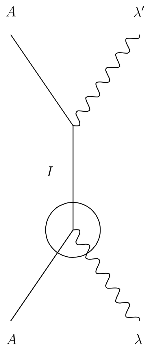
Figure 1:Feynman diagram for the first term under the sum in Eq. (2), which is resonant when for some intermediate state . At resonance, energy is conserved at the lower vertex (circled).
The resonant divergence of the scattering cross is nonphysical, so a number of questions are raised. First, what is wrong with our derivation of the Kramers-Heisenberg formula, that we obtain non-physical divergences, and how do we correct them? Next, how close to can we come before the Kramers-Heisenberg formula (47) breaks down? And finally, since we know the cross cannot really be infinite at resonance , how high does it go? Recall that for non-resonant frequencies, that is, that are not close to for any intermediate state , the Kramers-Heisenberg cross is of order . That is, it is of order in atomic units, which is very small by atomic standards. It is of interest to see by what factor this small cross is enhanced at resonance.
To see some of the qualitative features of the divergences in the Kramers-Heisenberg formula, consider the Feynman diagram of Figure 1. A question that arises is whether energy is conserved at the vertices of the diagram, for example, at the lower vertex (circled), where the energy of the initial state is and that of the intermediate state is . The answer depends on the photon energy but for most values of this parameter energy is not conserved. There is no reason why it should be, since the intermediate states originate in a resolution of the identity, which is a sum over all states, regardless of their energy. Nevertheless, the Feynman diagram suggests that somehow the initial state is transformed into the intermediate state at a certain time, which later transforms into the final state. In quantum mechanics energy is only precisely defined in processes that take an infinite amount of time, while for a process that takes time the energy is uncertain by an amount . In fact, intermediate states in Feynman diagrams only survive for a limited amount of time, or at least this is an interpretation that can be given to the machinery of the Dyson series developed in 34. Time-Dependent Perturbation Theory. Such a state is called virtual. For the lower vertex of the Feynman diagram in question, note that , so that is proportional to the resonant denominator we see in the Kramers-Heisenberg formula. The whole amplitude is proportional to , that is, it is proportional to the amount of time that the intermediate state is allowed to survive.
If is not near any resonant frequency for any intermediate state , then is of order unity in atomic units, so any given intermediate state survives only for a time of order unity before disappearing again. This means that the contribution of the state to the transition amplitude, which is computed in the Dyson series as an integral over time, can only accumulate to a small value before the virtual state disappears. The time integral in question is the one over in (38); the integrand has the phase factor , which in the context of the Kramers-Heisenberg formula is
If is not resonant, then the contribution to the transition amplitude just oscillates with a frequency and remains small.
If however we let approach a resonant frequency for some intermediate state , then gets smaller, the virtual state lives for a longer time, and the transition amplitude accumulates. This is reflected by the fact that the denominator gets smaller. As , it would appear that the virtual state could live for an arbitrarily long time, which would mean that it is becoming a real state.
But the intermediate state in question must be an excited state, since we are assuming that is the ground state, so it cannot live forever, rather it will eventually undergo the spontaneous emission of a photon and drop into a lower state. This will become a significant process when is comparable to , where is the lifetime of the excited state . is the usual symbol used for the decay rate of an excited state, measured in energy units. Thus we can expect that the predictions of the Dyson series and the Kramers-Heisenberg formula, as derived in 43. Scattering of Radiation by Matter, will break down when
As explained in 42. Emission and Absorption of Radiation, for E1 transitions is of order in atomic units, so the fraction of the axis over which the breakdown occurs is very small. For M1 and higher order transitions is even smaller. In other applications (nuclear physics, particle physics) may be relatively much larger (that is, broad resonances exist).
Time-dependent perturbation theory, as we have presented it in 34. Time-Dependent Perturbation Theory, is based on the method of successive approximations, in which a lower order approximation is substituted back into the Schr"odinger equation in the interaction picture and integrated to get the next approximation. It does not take into account the depletion of probability from the initial state due to the perturbation, so its validity is limited to short times, that is, . To cure the divergences in the Kramers-Heisenberg formula we need a theory capable of handling the long-time behavior of the system, that is, one that is valid for times .
Decay of an Excited State; the Decay Rate 
To analyze the long-time behavior of quantum systems, we will take a model problem, that of the decay of an atom in an excited state . We outline the problem in this , which contains a slight rephrasing of some of the material given in Spontaneous Emission. For the rest of this analysis we set except that we restore ’s selectively when it makes final formulas look more familiar.
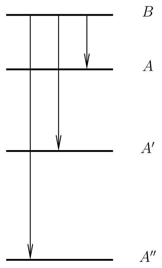
Figure 2:An atom in excited state emits a photon and drops into a lower state, of which there may be more than one (, , etc).
We assume the atom is initially in an excited state with no photons in the field, and that it subsequently makes a transition to a lower state with the emission of a photon. There may be more than one lower energy state to which a transition can be made, , , etc., as illustrated in Figure 2. As in 42. Emission and Absorption of Radiation{} we let the initial state be , where is the vacuum state of the field, and we let the final state be , that is, the state in which the atom is in state and there is one photon in the field of mode . We take the Hamiltonian to be
where , and are given by (5) and where we set as it is convenient to have a symbol for the entire perturbation.
According to first-order time-dependent perturbation theory, the transition amplitude in the interaction picture to find the system in state at time is
where is interpreted as
See (40) and (12). We note that can only change the number of photons by while can change them only by 0 or , so in (6) can be replaced by .
Squaring the transition amplitude to get a probability we have
where is the usual symbol we have used for an approximate -function, as defined by (51). Dividing this by and summing over final states gives us the transition rate, according to first-order time-dependent perturbation theory. If we want the total rate of decay, we must sum not only over all photon states but all atomic states . This gives
where we have taken long enough to replace the function by a genuine -function. There is no harm in summing over all states , including those higher in energy than , since for those the -function will give zero.
A -function is only meaningful under an integral, so when interpreting formulas such as (9) it must be understood that the sum on photon modes includes a sum on wavevectors of the photon, which in the infinite volume limit can be written as an integral over the frequency of the photon,
The volume factor will cancel when we compute the matrix element.
As noted in 42. Emission and Absorption of Radiation, this calculation of the decay rate really gives the slope of the decay curve at . See Fig.~\figr\radnmatt.1, in which the decay rate is denoted (the Einstein -coefficient) rather than . (The notation is appropriate for the decay rate to a specific final state, while is the decay rate to all possible final states.) First-order time-dependent perturbation theory is giving the probability of remaining in the initial state as
which is correct for but absurd for longer times. For longer times we might expect an exponential decay law but that is not proven by first-order time-dependent perturbation theory. We do have the first term in the Taylor expansion of the exponential,
but we haven’t proven that the higher order terms are the right ones.
To access the long-time behavior of the system it won’t help to go to higher order in time-dependent perturbation theory. These higher order terms will generate powers of , that is, a Taylor series expansion of the probability in time about . This is a poor way to understand the long-time behavior.
An Approach Based on Laplace Transforms and Green’s Functions
Let us return to the formalism of time-dependent perturbation theory in the general notation used in 34. Time-Dependent Perturbation Theory. We write the Hamiltonian as , and we let the initial state be
where is an eigenstate of ,
The state of the system at a later time is
where we have expanded as a linear combination of eigenstates of , , for simplicity assumed to be discrete. The expansion coefficients are the transition amplitudes in the Schr"odinger picture,
In this analysis we will work in the Schr"odinger picture, but for reference the transition amplitudes in the interaction picture, which we denote by as in 34. Time-Dependent Perturbation Theory, are related to those of the Schr"odinger picture by
See (30). The two amplitudes differ by a phase factor, so the transition probability, which is the square of the amplitudes, is the same in both pictures. Differentiating (16) with respect to time we obtain an evolution equation for the transition amplitudes in the Schr"odinger picture,
or,
This is really just a version of the Schr"odinger equation and it is exact.
We will solve (19) by means of Laplace transforms. A Laplace transform is essentially a one-sided Fourier transform, that is, the range of integration only goes from 0 to instead of to . (In comparison to the usual definition of the Laplace transform there is also the question of a deformation of the contour of integration in the complex plane, which we gloss over, the main point being that we will be using a one-sided Fourier transform.) The one-sided transform is necessary in our applications since we are interested in decay processes that go to zero as but which diverge as (and in any case we are only interested in ). The variable conjugate to is an energy-like variable, so we want to consider transforms like
The essence of this integral is
However, as discussed in The Outgoing Energy-Dependent Green’s Operator, this integral does not converge at the upper limit. To fix this we push into the upper half complex energy plane, making the replacement , where is a complex energy. Then the integral (21) gives the Green’s operator, to within constant factors. To get these right, we define the “Laplace transform” for our purposes as the integral operator
for . Then we have
where is the Green’s operator as defined by (58) (with ), and where we denote the Laplace transform of by .
The advantage of Laplace transforms is that they convert differential equations into algebraic equations, which are easier to solve, and they also deal nicely with initial conditions and transients. This is like the method of complex impedances when analyzing an electrical circuit, which is much easier than solving coupled differential equations for the currents and charges in the circuit elements.
Applying the Laplace transform to the left-hand side of the Schr"odinger equation (19) and integrating by parts we obtain
Note that . Applying the Laplace transform also to the right-hand side of (19) we obtain
This is an algebraic equation for the Laplace transforms of the transition amplitudes that is equivalent to the Schr"odinger equation and is still exact.
We can obtain the same result by noting that
so that
Now sandwiching this by on the left and on the right, we obtain
which is the same as (25).
Solving for the Transition Amplitudes
We now apply these results to the decay problem described in \secrnlw-2, making the identifications , , , and . Also, we make the approximation of working on the subspace of the ket space spanned by and , ignoring all states with two or more photons. This means that we interpret the resolution of the identity as
We can enlarge this space to get a better approximation, at the expense of solving a more complicated system of equations.
We specialize (25) to the case , which for our decay problem means that the final state is the same as the initial state . The corresponding amplitude is , the amplitude to remain in the initial state. Making the replacement (29) for this case we obtain
Taking into account the numbers of photons that and can create or destroy, we can write this as
Similarly, taking the case and identifying with , so that , we can write (25) as
where we have restricted the resolution of the identity as in (29).
Equations~(31) and (32) are algebraic equations for the Laplace transforms of the transition amplitudes, and . The various terms can be assigned an order in the perturbation , where we count as of order . The amplitude is of order unity in the perturbation, since it is non-zero even when , as shown by (31). Then since the matrix element is of order , we see from (32) that the amplitude is also of order . This also follows from the fact that transitions to the states are induced by . From this it follows that the final term in (32) is of order . As for (31), its terms are of at most second order in .
We will work to second order in the perturbation, neglecting the final, third order term in (32) (the final sum). This allows us to solve for the amplitude in terms of ,
We substitute this back into (31), which allows us to solve for the amplitude ,
where we define
The symbol stands for “denominator.” Finally, we can substitute this back into (33) to obtain
Equations~(34) and (36) are explicit solutions for the Laplace transforms of the transition amplitudes and . We must now carry out the inverse Laplace transform to get the amplitudes themselves.
Inverting the Laplace Transform
Let us revert to a general notation, denoting transition amplitudes by and their Laplace transforms by . To carry out the inverse Laplace transform we consider the integral
where is a contour that runs just above the real axis in the complex energy plane, as illustrated in Figure 3. The essence of this integral is
If then the integrand is exponentially damped in the upper half plane, and the contour can be closed by a semicircle at infinity which does not contribute to the integral, as illustrated in Figure 4. This contour encloses no singularities since is analytic in the upper half plane, so the value of the integral is zero.
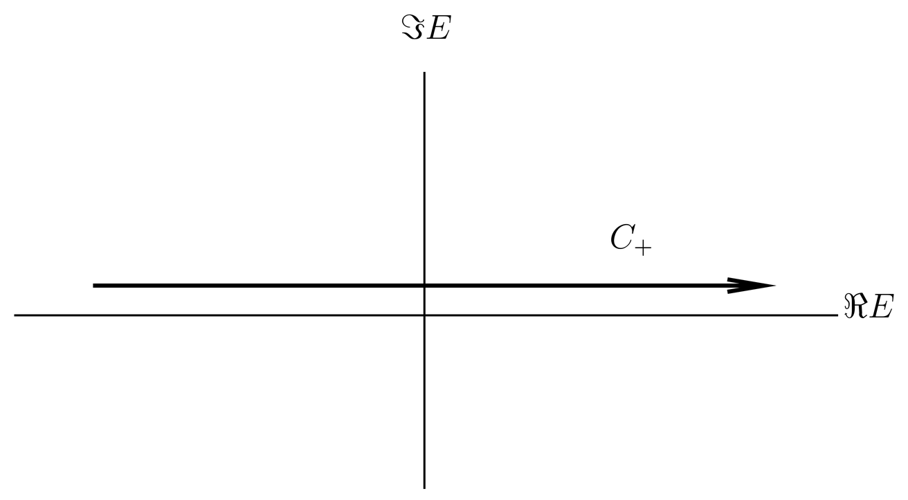
Figure 3:The contour , used in the inverse Laplace transfrom, runs just above the real energy axis.
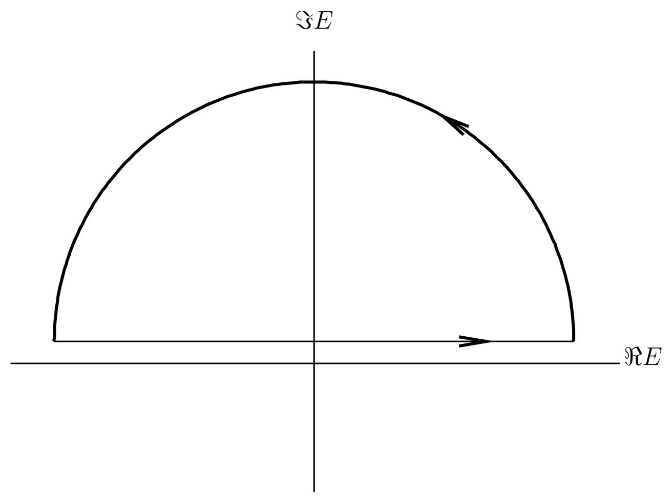
Figure 4:For negative times the contour can be closed in the upper half-plane.
For positive times the integrand diverges exponentially in the upper half-plane so we cannot close the contour there. Nor can we close it in the lower half-plane, since that would involve crossing the real energy axis where has singularities (poles and branch cuts). To evaluate the integral (38) for positive times we consider a different integral,
where runs just below the real energy axis, as illustrated in Figure 5. For positive times the integrand damps exponentially in the lower half-plane, so the contour can be closed as in Figure 6. But since is also analytic in the lower half-plane, the integral (39) vanishes for .
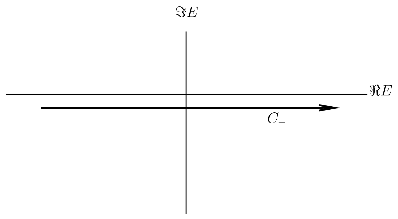
Figure 5:The contour runs just below the real energy axis.
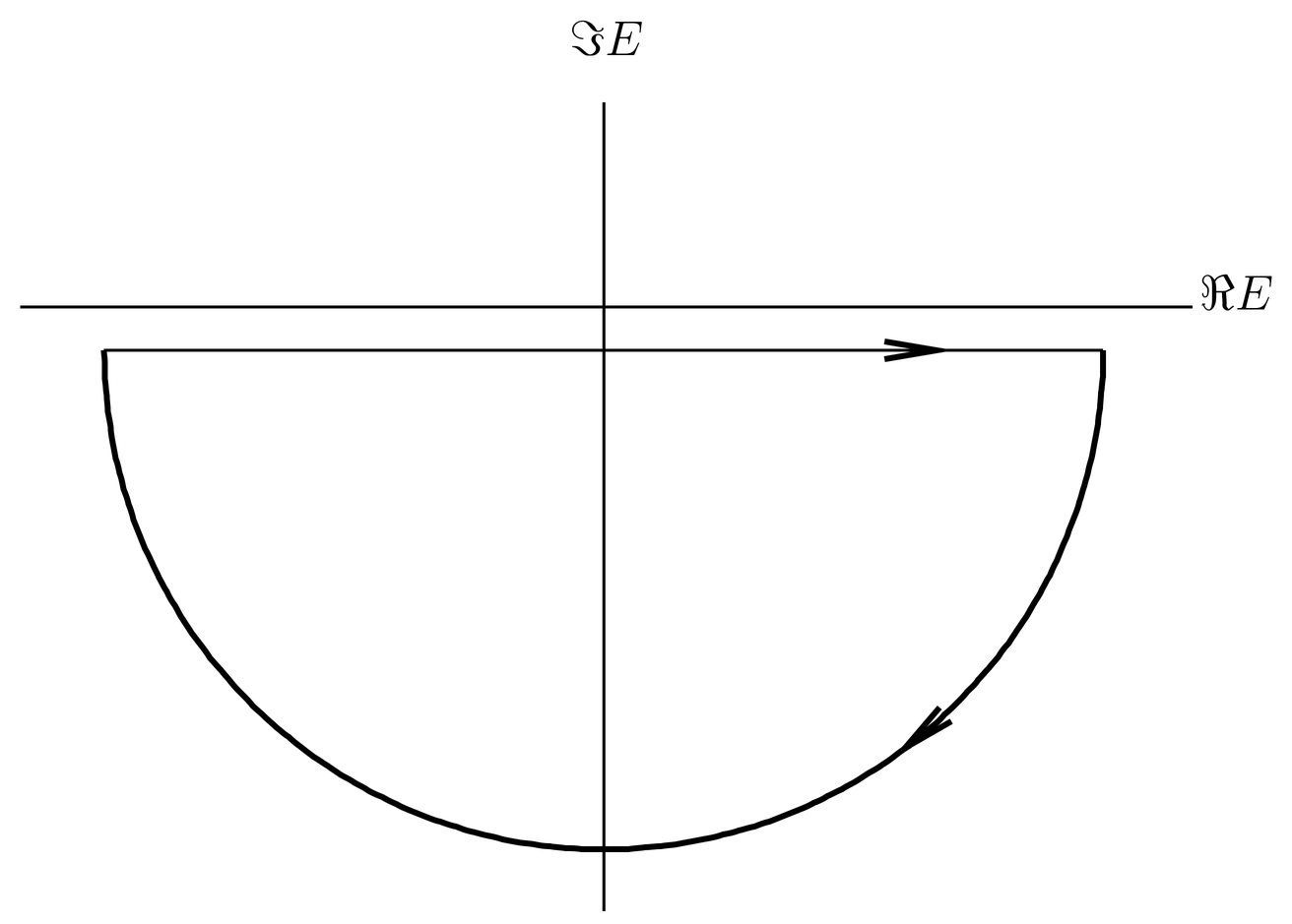
Figure 6:For positive times the contour can be closed in the lower half-plane.
To return to the integral (38) for positive times, we can subtract the integral (39) without changing the value since the latter is zero. That is, for we have
where as the contours and are pushed toward the real axis we get an integral running over the real axis itself, in which the integrand contains the difference in just above and just below the real axis. But this is the discontinuity in the Green’s operator across the real axis, which is . See (73) and (77). Thus the integral (40) becomes
Altogether, we have
and the inverse Laplace transform of the transition amplitude is
Transition Amplitude in the Unperturbed System
Now we apply the inverse Laplace transform to the amplitudes and , given by (34) and (36). We start with the amplitude to remain in the initial state ,
Before doing this in full detail, let us neglect the terms of seen in (35) that involve the perturbing Hamiltonians and , in order to see the evolution due to the unperturbed system. We do this to gain some experience and confidence with the formalism.
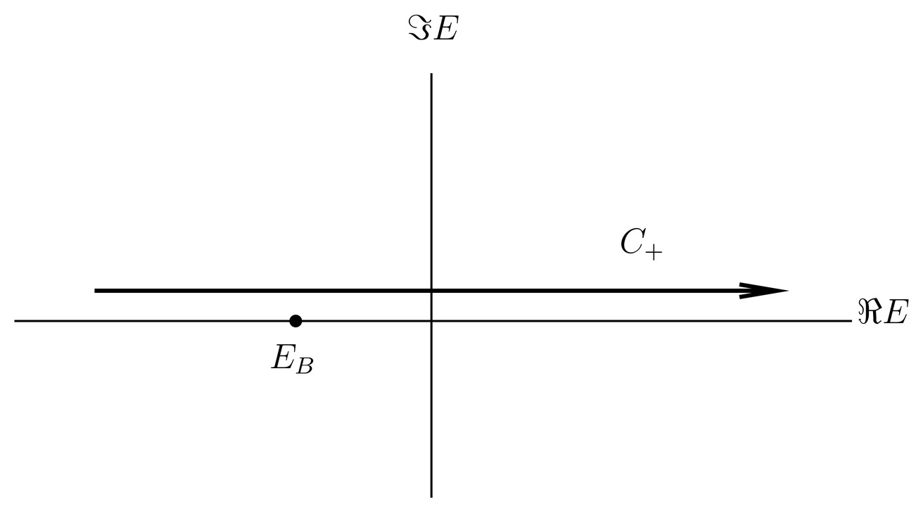
Figure 7:Complex plane for the inverse Laplace transform for the unperturbed approximation to . The integrand has a simple pole on the real axis at .
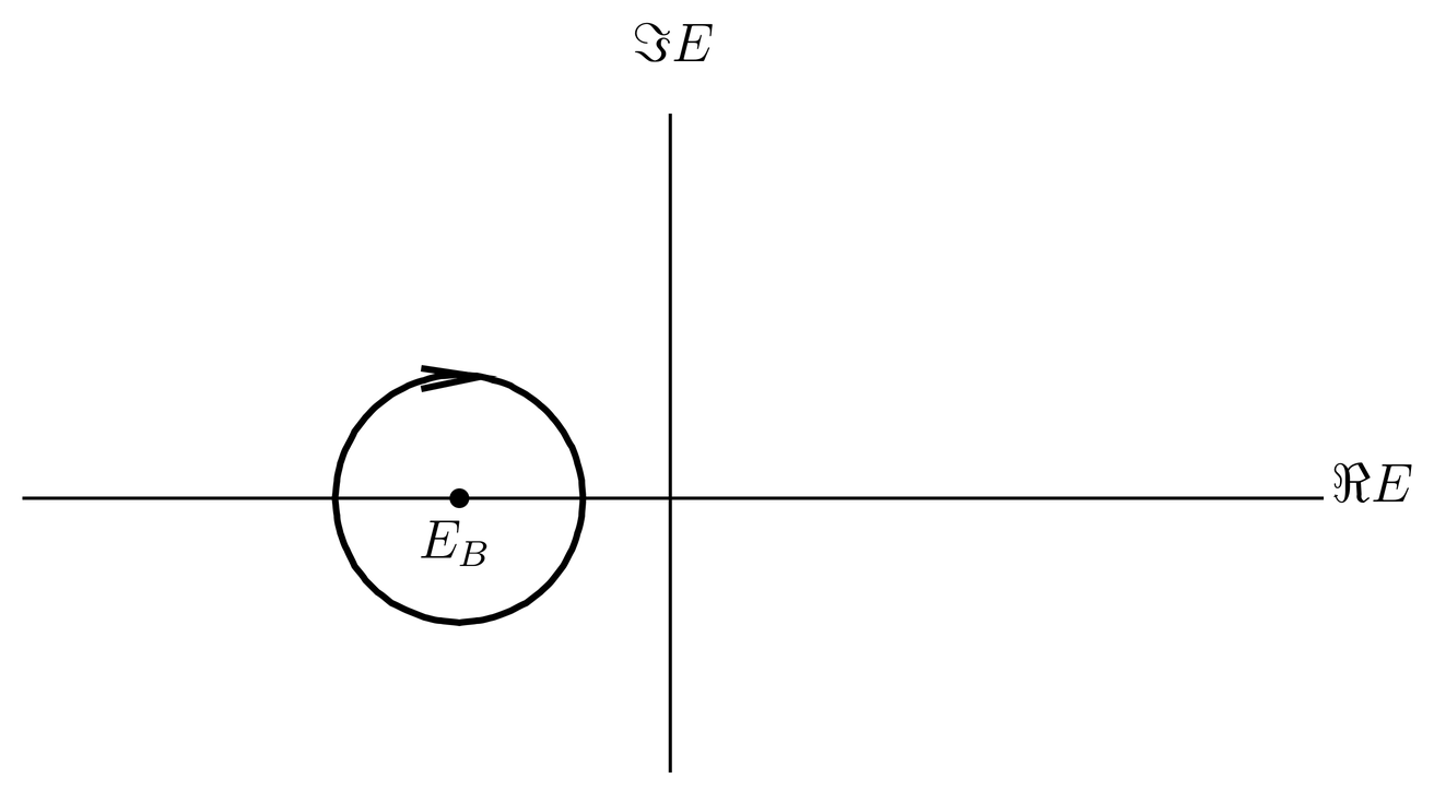
Figure 8:The contour of Figure 7 can be closed in the lower half-plane and contracted around the pole.
In that case becomes simply , and we have
The integrand has a pole on the real axis at and no other singularities. For the contour can be closed with a semicircle in the lower half-plane and can then be contracted into a small circle running in the clockwise (negative) direction around the pole. See Figs.~Figure 7 and Figure 8. Then by the residue theorem we have
which is exactly the time evolution we expect for the amplitude to remain in the initial state when there is no perturbation. We see that the time dependence of the amplitude depends on the location of the poles of the integrand of the inverse Laplace transform.
Denominator on the Real Axis
To handle the full expression (35) for let us first set for a point on the contour ,
where we have changed the sign of the denominator of the last term and compensated with the overall sign of that term. We remember that actually implies the integral (10) over .
We want to let in this expression to get on the real axis, but the final term is tricky. It looks like we could just set in this term and we would obtain a quantity that was purely real, but this is incorrect. In fact, if we just set we get an integral that has the mathematical form
where is a smooth function and where the interval straddles the singularity at . (The variable in the integral (48) is like in the integral (47).) The problem is that the integral (48) is not defined. The part of the integral from to diverges with one sign and the part from to diverges with the opposite sign. Thus the integral has the form , and is not defined.
We cannot just set in an expression like (47), instead we must take the limit . That is, we have something of the form
Assuming is real, the real and imaginary parts of this integrand are obtained from
As for the imaginary part, as we get a representation of the -function,
so the imaginary part of the final sum in (47) is nonzero as and is given by
A bare formula like (51) is not meaningful if interpreted as the limit of a function, since the so-called “-function” is not a real function. It does not make sense to say that the -function is zero everywhere except at one point where it is infinite, and that its integral is unity. Instead a formula like (49) must be understood as being used under an integral sign, in which the left-hand side is integrated against a smooth function and the limit is taken. The “-function” is an example of what is called a distribution, something that can be regarded as the limit of a family of functions used under an integral.
There are other distributions besides the -function, in fact, the real part of (50) is another example which is denoted
This is called the “principal value” of . This equation is a “bare” formula like (51). Its real meaning is
Without the the left-hand side of this equation would not be defined, as explained above.
Now we can take the limit to push down onto the real axis. We write
where
The Zero of and the Complex Energy of State 
The zero of is the pole of the integrand of the inverse Laplace transform (44) and is important for evaluating that integral. It also turns out to be a kind of complex energy of the state , once the perturbation is turned on. In the unperturbed system has a zero on the real axis at but when the perturbation is turned on is nonzero everywhere on the real axis because the imaginary part is positive there. Thus the zero must have moved to some complex location nearby. We denote the zero by , so that . We write so that is the shift in the zero of due to the perturbation. To find we write
Assuming is small we neglect it in the last two terms which are already small, finding
or,
where we have rearranged signs in the third term. We see that the zero of has moved off the real axis into the lower half plane. As for its imaginary part, a comparison with (9) shows that it is , where is the decay rate of state .
The real part of bears a close relationship to the energy shifts of bound state perturbation theory, as explained in 23. Bound-State Perturbation Theory. The state is a bound (normalizable) eigenstate of with energy . It is an eigenstate of the unperturbed system, that is, the atom with the interactions with the electromagnetic field switched off. Of course, in reality we cannot switch off those interactions; do they lead to shifts in atomic energy levels?
To answer this question we consider using bound state perturbation theory to compute the shift in level due to the perturbation . According to (26), there is a first order shift
where does not contribute. Also, according to (27) the nominal second order shift is
If we replace by to get the lowest order contribution, then the only states that we need sum over are the single photon states , and we obtain
This is almost the third term on the right in (59), missing only the principal value sign.
Actually, without the principal value in (62) is not defined, nor is it justified to use bound state perturbation theory to find the energy shift in the state due to the interaction with the electromagnetic field. Bound state perturbation theory applies when we have discrete energy levels that are separated from one another, and in this system the state is a discrete state imbedded in the continuum. Nevertheless, our search for the zero of has led to expressions that are obviously related to the energy shifts of bound state perturbation theory, except that the answers are well defined and the energy shift includes an imaginary part. Let us therefore simply define to be the third term on the right in (59) (that is, by (62) but with a principal value sign), so that
where
Then is the real part of the energy of atomic state , corrected for interactions with the field, while the imaginary part is .
The Transition Amplitude and the Exponential Decay Law
We return to the integral (44) for the transition amplitude . The integrand has a pole at , located near and below the energy of the unperturbed state , as illustrated in Figure 9. The contour can be closed with a semicircle in the lower half plane and can then be contracted into a small circle around the pole at in the lower half plane.
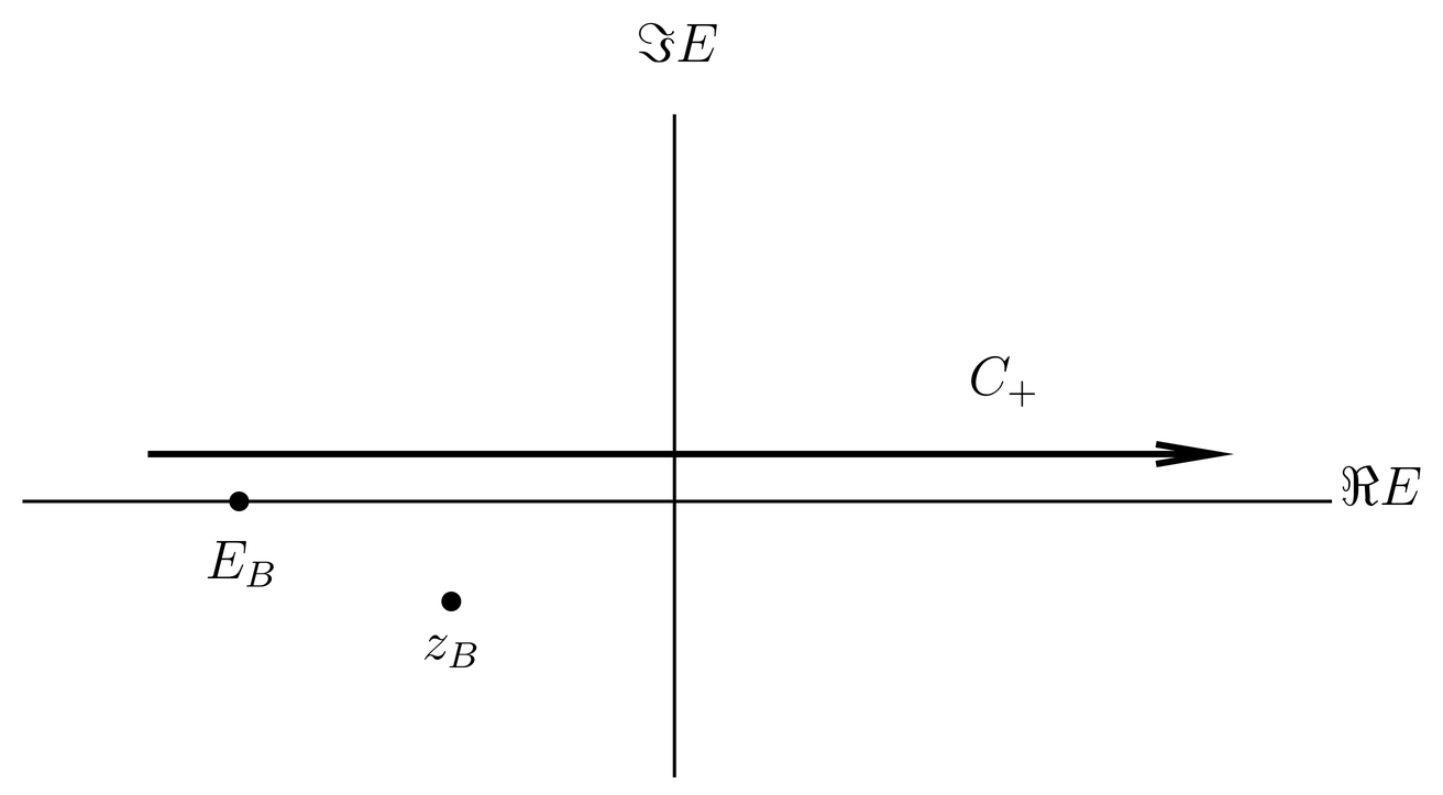
Figure 9:Complex plane for the inverse Laplace transform for , Eq. (44). The integrand has a simple pole at , near and below the unperturbed energy .
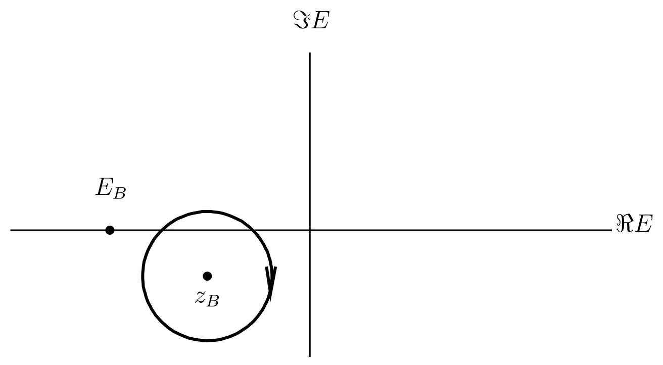
Figure 10:The contour of Figure 9 can be closed in the lower half-plane and contracted around the pole at .
Near we can expand ,
But the first term vanishes and by (35) we have . Therefore to lowest order,
when is near . The contour in Figure 10 can be contracted arbitrarily close to the pole at so the integral (44) can be written
where the circle is traversed in a clockwise (negative) direction. We can also write this as
This shows that the amplitude to remain in the initial state evolves with a real phase factor indicating an energy , that is, one corrected for the interactions with the field, but with an exponential decay factor. The probability to remain in the initial state is the square of the amplitude,
which shows the exponential decay law.
We see that the exponential decay law is not a rigorous consequence of the Schr"odinger equation, but rather it follows from a series of nontrivial approximations. In fact, it is known that there are deviations from the exponential decay law for long times.
The unperturbed system has a genuine bound state at but when the perturbation is turned on there is only a continuous spectrum in the neighborhood of . The discrete state has “dissolved into the continuum,” and become a resonance. A similar mechanism explains the resonances associated with the doubly excited states in helium, as discussed in The Doubly Excited States.
This derivation has been based on a model of an atom, but it applies in its essence to the decay of any excited state of a system, including radioactive decays of nuclei and decays of unstable particles. The derivation looks complicted, but that is because the exponential law is not exact. The usual “simple” derivations of the exponential decay law rely on a type of statistical assumption of the Markov type, which means that the transition probability for a system depends only on the present state and not the previous history. This is what we usually assume about radioactive decay. For example, if a nucleus has not decayed after ten times its average lifetime, the probability that it will decay in the next second is the same as it always was. The nucleus does not try to “hurry up and decay” because it has failed to do so for so long. At least this is what we usually assume. But studying the decay by solving the Schr"odinger equation, we find that the exponential decay law is only approximate. Various aspects of this situation are discussed in an appendix to the first edition of Sakurai’s book, Modern Quantum Mechanics.
The Transition Amplitude 
We can also get the amplitude to make a transition from the initial state to some specific final state . According to (36) this is
The matrix element is independent of and can be taken out of the integral. As for the rest of the integrand, it has poles at and at , as illustrated in Figure 11. The figure is drawn for the case , as required if there is to be a transition .
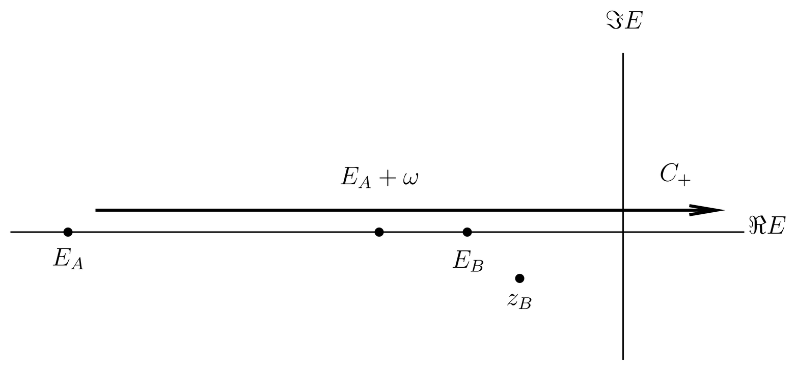
Figure 11:Complex plane for the inverse Laplace transform for , Eq. (70). The integrand has poles at and at .
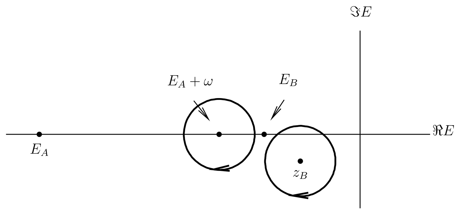
Figure 12:The contour of Figure 11 can be closed in the lower half-plane and contracted to two small circles around the poles at and .
Evaluation of the integral by the residue theorem gives two terms, one for each pole,
This is valid for any final state but the amplitude will be small unless energy is approximately conserved, which means that is near to , and therefore near to . If this is the case then (66) gives
where we define
Then the two denominators in (71) are the same to within a sign and the result can be written
Amplitude and Probability as 
The long-time behavior of the system is of interest but as the amplitude oscillates and does not approach a limit due to the phase factor . This factor is due to the evolution under the unperturbed Hamiltonian , which is all that matters at long times because the photon will have left the atom behind and is no longer interacting with it. A similar situation holds in scattering theory, in which a wave packet directed at a target evolves according to the free particle Hamiltonian at large negative and large positive times. See the discussion in The -Matrix.
If we switch to the interaction picture this time evolution is stripped off, and the amplitude is
This is the same result we got with time-dependent perturbation theory, see (6) and (7), except that is replaced by . The transition amplitude in the interaction picture does have a long-time limit,
whose square gives the long-time probability,
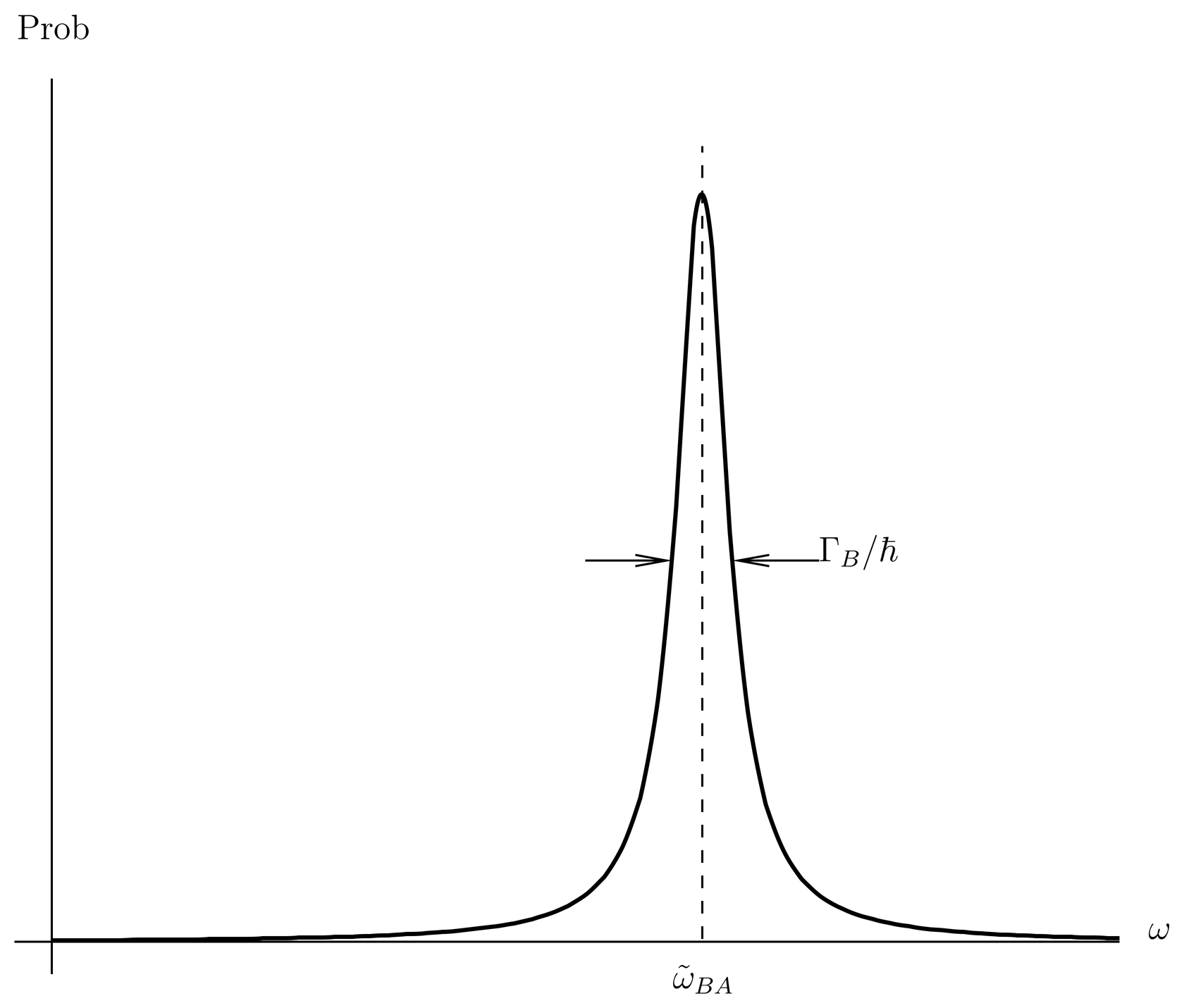
Figure 13:The transition probability has a Lorentzian dependence on the frequency. The peak is centered at the resonance frequency and its full width at half maximum is . ure is not to scale.
The correction term in the denominator does not matter much if , but when the transition probability varies rapidly in . The matrix element may also depend on but is nearly constant over the small range of order about resonance. Overall the dependence of the transition probability has the Lorentzian shape, with a full width at half maximum (FWHM) of . See Figure 13.
The Lorentzian replaces the energy-conserving -function that we had with time-dependent perturbation theory. The photons emitted in the transition do not all have the same energy, but rather there is a spread of order . Note the scales in the figure. In a typical atomic problem is of order unity in atomic units, while for E1 transitions is of order .
The width is what is called the natural line width of the spectral line . Other effects also contribute to the broadening of the spectral line, for example, Doppler shifts if the source is a gas. Doppler shifts broaden the spectral line with a Gaussian profile, because of the Maxwellian distribution of particle velocities. If the density of the gas is above a certain amount there will also be pressure broadening, caused by the fact that before the atom has a chance to decay it has a collision with another atom. This effectively resets the clock in the evolution of the state of the atom. With pressure broadening the width of the spectral line can still be written , except that now is the collision time instead of the lifetime for spontaneous emission. The natural line width is the minimum line width obtained when all other sources of broadening are eliminated.
You may wonder why in the formula (73) for we correct the energy for interactions with the field but not . Actually we should correct both energies but our formalism has not done this since we have restricted the ket space to states with at most one photon. Notice that if is the ground state its lifetime is infinite so , but could be an excited state lying between and the ground state, as illustrated in Figure 2. We would need a more sophisticated model to take into account the decay of both states and such a excited state . This is required, for example, in problems of optical pumping or photon cascades. If is also an excited state then the line shape of the transition is a Lorentzian with FWHM given by .
As the atom drops into the state with probability, so the sum of all the probabilities (77) should add to 1. We can see that it does if we make the replacement,
which follows from the representation (51) of the -function and the fact that the matrix element is slowly varying over the energy range . This gives
as follows from (9).
Fixing the Kramers-Heisenberg Formula
Now we can see how to fix the singularities in the Kramers-Heisenberg formula. As noted in \secrnlw-1, the vanishing denominators arise from the time integrals in the Dyson series. For the resonant terms in question, the phase factor that is integrated is given by (3), which we write here as
dropping the primes on and setting . The two time-dependent exponential factors shown came from a matrix element which in the case of the Kramers-Heisenberg formula can be written
where the factors of represent the switch from the interaction picture to the Schr"odiner picture. From another point of view they also represent the time evolution of the states of the system at a lower order approximation that is being substituted back into the Schr"odinger equation and integrated over time to get the next order approximation.
Based on what we have done with the long-time behavior of quantum systems, however, it would be more accurate to use the time evolution of states and corrected for the interactions with the field, that is, to replace the factor (80) by
where
as in (64). We do not include a term because in our outline of the problem in \secrnlw-1 we assumed that was the ground state of the atom.
If we do this, then the denominator of the Kramers-Heisenberg formula (1) is replaced by
where
(like (73) but with both energies corrected). It is logical that the resonance frequency should be corrected in this manner, because the real resonance occurs at , not . Also, the denominator now has an imaginary part and does not vanish at . We see, as suspected in \secrnlw-1, that the nominal Kramers-Heisenberg formula breaks down when . Near such frequencies the amplitude sum (2) is dominated by a single term, and
The cross is given by
If the transition is allowed as an E1 transition, then is of order in atomic units, so that at resonance the cross saturates at a value that is of order times larger than it is out in the “desert” where is not close to any . In terms of powers of the fine structure constant, the cross is of order at resonance, which is quite large by atomic standards. This is of the order of the square of the wavelength, which is characteristic of resonant cross s in general.
Thus the cross as a function of frequency has the Lorentzian shape in the neighborhood of a resonance, much like the sketch in Figure 13. The width of the resonance is of order and the height is of order , so if a gas is subjected to broad band radiation then by far the majority of the scattering is resonant, at least until the beam is depleted of resonant photons. This is the reason for the dark Fraunhoffer lines in the solar spectrum; as light from the sun passes through the cooler, outer layers of the atmosphere of the sun, the resonant photons are scattered into random directions and removed from the direct sunlight. In this process, the Doppler shift from the motion of the atoms causes the dark lines to be broadened considerably in comparison to the natural line width.
It was realized by the mid-nineteenth century that the dark Fraunhoffer lines in the spectrum of the sun or other stars occur at the same frequencies as the emission spectra of various elements, and so can be used to determine the chemical composition of stellar atmospheres. The element helium was first discovered in this way in the sun’s atmosphere, before it was known on earth (hence the name, from Greek “helios” meaning “sun”).