40. The Classical Electromagnetic Field Hamiltonian
Introduction
In these notes we motivate the necessity for quantizing the electromagnetic field, we outline a procedure for doing that, and then we carry out the classical part of that procedure, which is to find a classical Hamiltonian for the combined system of matter plus electromagnetic field. In a subsequent set of notes we shall quantize this classical Hamiltonian and study the results. Standard references for the material in these notes include Heitler, The Quantum Theory of Radiation and Cohen-Tannoudji, Dupont-Roc and Grynberg, Photons and Atoms.
The Electrostatic (Coulomb) Model, its Limitations and Generalizations
So far in this course we have mostly used an electrostatic or Coulomb model to describe the interactions of charged particles with one another. In this model, a charged particle responds to the electric field evaluated at the position of the particle, where the electrostatic potential is determined by the instantaneous (non-retarded) positions of all the other charged particles. The potential , where is the charge of the particle, enters into the particle Hamiltonian. This model omits a number of important physical effects, including the magnetic fields produced by the moving charges, the effects of retardation (finite velocity of propagation of signals between the charged particles), and radiation.
If the velocities are low and the distances between particles not too great, then the dominant (quasi-static) part of the magnetic interactions between charged particles can be taken into account by adding certain velocity-dependent terms to the classical Lagrangian, resulting in the so-called Darwin Lagrangian. In the Darwin Lagrangian, magnetic fields are treated in a similar manner to electrostatic fields: the magnetic field at some (field) point in space is determined by the instantaneous (nonretarded) positions and velocities of the charged particles. We will not use the Darwin Lagrangian explicitly in this course, but its spirit was very much with us when we computed the spin-orbit corrections to the atomic Hamiltonian in 25. Fine Structure in Hydrogen and Alkali Atoms. In multi-electron atoms, there are other effects of a similar nature, for example, the orbital motion of one electron is influenced by the force due to the magnetic field produced by the motion of the other electrons. These effects are small (they are part of the fine-structure terms), a sign that the electrostatic model is a good first approximation.
In both the electrostatic and Darwin models, the fields are definite functions of the instantaneous (non-retarded) particle positions and velocities, so the dynamics of the particles can be described by a Hamiltonian containing only the particle degrees of freedom. Only Hamiltonians of this sort have been considered up to this point in this course. These models, however, are incapable of representing effects such as retardation and radiation.
As for retardation, its effects are small for nonrelativistic systems of small spatial extent, so the electrostatic model is often quite a good one, but the question remains as to how we would treat those effects if we wished to. In fact, in multielectron atoms retardation effects are of the same order as the fine structure, and must be taken into account for a fully satisfactory theoretical treatment of the fine structure.
Radiation is also a small effect in ordinary atoms, in the sense that the probability of emitting a photon is small during a single rotational period of an electron in an excited state. Nevertheless, over a large number of rotational periods radiation becomes a near certainty, and an atom in an excited state will make a transition to a lower energy state. But there is no hint of this in the electrostatic or Darwin models, either in classical mechanics or in quantum mechanics. For example, in quantum mechanics, these models predict that excited states of atoms are stationary states, that is, energy eigenstates, with an infinite lifetime. Similarly, in classical mechanics in the electrostatic model two charged particles orbit each other in Kepler ellipses forever without emitting any radiation. The inclusion of magnetic effects through a Darwin model modifies the orbits but does not lead to radiation.
In books on classical electromagnetic theory, there are typically two kinds of problems encountered. In one, the electromagnetic field is given and it is desired to compute the trajectories of the particles that respond to this field. In the other, the currents and/or charges are given, and it is desired to compute the fields produced. For example, this is how the radiation field produced by accelerated charged particles is usually computed: One assumes that the trajectory of a charged particle is given, with given velocity and acceleration at any instant of time. This implies a certain charge and current density in space, which are then used as sources in Maxwell’s equations, from which the total fields can be computed. These fields are dominated by radiation at large distances, while for low velocity particles at short distances they are dominated by non-retarded Coulomb or Coulomb-plus-Darwin fields.
In reality, however, fields and the particles act on each other, and the dynamics of the combined field-particle system must be solved for a fully realistic account. This is not an easy problem in classical electrodynamics, which explains why books on the subject usually avoid it or simplify it in various ways. There are no nontrivial exact solutions of the equations of motion for the coupled field-particle system, and approximate solutions require some small parameter. We shall find a similar situation in quantum mechanics as well, where fortunately for our applications there is a small parameter (the fine structure constant ) that serves as a perturbation parameter.
Moreover, at the classical level there is a fundamental difficulty with the formulation of the interactions of charged particles with electromagnetic fields, namely the infinite self-energy of a point particle. This difficulty cannot be cured at the classical level, and all classical models that incorporate the point nature of charged particles are ultimately inconsistent. These infinities played a central role in the history of quantum electrodynamics, as we shall explain below.
These considerations indicate that in order to incorporate effects such as retardation and radiation into quantum mechanics, it will be necessary to describe the coupled dynamics of the matter plus the field. This cannot be done with a Hamiltonian that contains only the matter degrees of freedom; instead, it will be necessary to include the field degrees of freedom as well. Doing this, however, requires some additional formalism, so in introductory courses in quantum mechanics the emission and absorption of radiation is usually discussed within a simplified model that we now describe.
The Semiclassical Theory of Radiation
In classical mechanics a charged particle responds to the forces produced on it by an electromagnetic field, absorbing energy from the field and returning some energy back to it in the form of radiation. Thus the field is modified by the presence of the particle. But if the field is strong it may be possible to ignore the effect of the particle back on the field, and to treat the particle as if it were moving in some given field.
Similarly, in quantum mechanics we can study the effect of a strong electromagnetic field on a system of charged particles by assuming that the fields are given functions of space and time, with given “external” potentials and . We do not worry too much about the sources of the external fields in such applications, because we ignore the reaction of our system back on those sources, which are not included as a part of the system under consideration. For example, we may consider an atom interacting with a light wave produced by a laser, or a magnetic field produced by currents in a coil. In such cases, the effects of the external field on a quantum mechanical system of charged particles is described by incorporating the external potentials and into the particle Hamiltonian. This is what we did in studying the Stark and Zeeman effect in 24. The Stark Effect in Hydrogen and Alkali Atoms\ and \zeeman, and spin precession in 14. Spins in Magnetic Fields.
If the external field is a radiation field, then the model is called the semiclassical theory of radiation, since the matter is treated by quantum mechanics but the field is treated classically. We studied an example of the semiclassical theory of radiation in our treatment of the photoelectric effect in 35. The Photoelectric Effect. That will be the only example considered in this course.
The semiclassical theory of radiation can describe rather easily the absorption of radiation by systems of charged particles, since the particles just respond to the forces of the external field, which changes their dynamical state. This is how we used this theory in our study of the photoelectric effect. It is not so easy to describe the emission of radiation within the semiclassical theory of radiation, but that can also be done in an ad hoc manner. The procedure involves combining the results for absorption with some kinetic theory (in the form of the Einstein - and -coefficients), statistical mechanics, and random phase assumptions. In this manner one can calculate the rate of emission of radiation (the power emitted) by a system of charged particles, both in the presence of an external field (stimulated emission), and in its absence (spontaneous emission). The argument is tricky and convoluted, and ultimately inconsistent, since the currents produced by the quantum system are ignored in Maxwell’s equations. Nevertheless, the semiclassical theory of radiation is definitely useful, and you will doubtlessly see it again if you study quantum optics or related subjects.
At a more fundamental level, however, the semiclassical theory of radiation is definitely unsatisfactory. Even if it were possible to restore self-consistency in the emission and absorption of radiation (to include the quantized particle currents and charges as sources of the field), the problem remains that the field is treated by classical mechanics, that is, the classical Maxwell equations, while the matter is treated by quantum mechanics. Thus we have a system in which some degrees of freedom are treated classically, while other are treated quantum mechanically. Any such hybrid classical-quantum model leads immediately to interpretational difficulties, for example, by making measurements on the classical degrees of freedom it becomes possible to violate the uncertainty principle in the quantum degrees of freedom. In the present case, if we can measure a classical electromagnetic field at a given point of space and time with arbitrary precision (the usual assumption in classical electromagnetic theory), then we can identify the position and velocity of the charged particle that produced that field to arbitrary precision. In actuality, measurements of field strengths are made by observing the forces on charged particles, which themselves obey the laws of quantum mechanics. The implications of quantum mechanics for the measurement of electromagnetic field quantities were examined in a famous 1933 paper by Bohr and Rosenfeld (English translation available in Quantum Theory and Measurement, by J. A. Wheeler and W. H. Zurek), which is a primary reference for these kinds of questions.
The Necessity of Quantizing the Electromagnetic Field
Thus we cannot expect that any hybrid classical-quantum model will bring us enlightenment into the fundamental physics of the interactions of charged particles and electromagnetic fields. Instead, we expect that a proper understanding will require that both field and matter be treated by quantum mechanics. We know how to do this for the matter, at least in the nonrelativistic approximation, but the usual (classical) description of the electromagnetic field as a field of -numbers (the values of and that can be measured with arbitrary precision) must be replaced by a quantum description.
We can already see some outlines of the resulting theory without doing much work. For example, one of the postulates of quantum mechanics is that every measurement process corresponds to a Hermitian operator acting on some ket space, and that the possible outcomes of the measurement are the eigenvalues of that operator. These outcomes are assigned probabilities by the rules of quantum mechanics, which describe the statistical results of measurements on an ensemble of identically prepared systems. In addition, in general different observables are not compatible, that is, they cannot be measured simultaneously with infinite precision. See 02. The Postulates of Quantum Mechanics\ and \density. Thus we must expect that in the quantum theory of the electromagnetic field, measurements of and are associated with some operators that act on some ket space, and that these measurements will exhibit statistical fluctuations and obey some uncertainty relations. In the quantum theory of the electromagnetic field, the -number (real-valued) fields and that form the basis of classical electromagnetic theory are replaced by operator-valued fields (actually, vectors of operators). These will be our first examples of quantum fields.
Now a few remarks about the history of quantum electrodynamics. Quantum mechanics was born in 1900 with Planck’s derivation of the correct formula for the black body spectrum. Although no one at the time fully understood Planck’s result, nevertheless it was clear that the electromagnetic field must obey some kind of quantum laws that are distinct from those of classical electromagnetic theory. Indeed, the classical theory predicts an “ultraviolet catastrophe,” that is, an infinite energy density, for radiation in thermal equilibrium with a heat bath. It was not until 1925 that the first reasonably complete formulation of quantum mechanics came about, and almost immediately, in two papers in 1926, Jordan made the first attempts at quantizing the electromagnetic field. By 1927 Dirac had laid out the basis of quantum electrodynamics, much as we shall study it in this course. This early version of quantum electrodynamics gave physically meaningful results for the interactions of charged particles with the electromagnetic field at lowest order of perturbation theory. These results were able to explain a wide array of phenomena involving the interactions of matter with radiation.
Subsequent developments were not all smooth sailing, however. By the early 1930’s it had become apparent that quantum electrodynamics, as it was then understood, led inevitably to infinities in higher order perturbation theory. Some of these infinities were quantum versions of the infinite self-mass of the point particle that had already been a problem in classical electrodynamics, but in addition it turned out in the quantum theory that particles have an infinite charge. These difficulties were a major preoccupation of theoretical physics during the first twenty years of quantum electrodynamics (roughly 1927 to 1948). Some physicists thought that the classical theory should first be cured of its infinities before applying quantum mechanics, while others thought that quantum mechanics itself should be replaced by a more fundamental theory. In the end, it turned out that quantum mechanics, combined with an insistence on relativistic covariance and gauge invariance, led to a set of rules for consistently removing the infinities from quantum electrodynamics to all orders of perturbation theory. This was the renormalization program due to Feynman, Schwinger, Tomonaga and Dyson. We shall cover some of the basic ideas of renormalization later in the course, when we study Bethe’s derivation of the Lamb shift. The result is the modern theory of quantum electrodynamics, which has served as a model for the quantum theory of other fundamental interactions (for example, quantum chromodynamics or QCD, the modern theory of the strong interactions, or the electroweak theory, which unifies the electromagnetic and weak interactions, both of which reached maturity in the 1970’s). See the book QED and the Men Who Made It, by Silvan Schweber, for more details about the fascinating history of quantum electrodynamics.
Granted that we must quantize the electromagnetic field, the question is how to do it. More generally, given a classical description of any dynamical system, how do we go over to the proper quantum mechanical treatment? No deductive procedure can be given, since quantum mechanics has more physics in it than does classical mechanics, and in fact this is often a nontrivial question. For example, although the classical theory of the gravitational field (Einstein’s general relativity) has been known for over a hundred years, it is still not certain what the correct quantum version of this theory should be.
Nevertheless, if we follow the procedure that is known to work for nonrelativistic material systems, it would run something like this. First we find the classical equations of motion, which we write in the form , where the ’s are the generalized coordinates of the classical system. This is basically a version of Newton’s laws (). Next we find a classical Lagrangian that gives the classical equations of motion as the Euler-Lagrange equations. Next we convert the Lagrangian into a classical Hamiltonian , by means of the Legendre transformation. Finally, we use the prescription of Dirac, which replaces the ’s and ’s of the classical system by operators satisfying the canonical commutation relations, . This last step is not unique, because multiplication of classical observables is commutative, while that of quantum observables is not, and in any case there may be physical effects of a quantum nature that are not suspected at the classical level (for example, spin). The validity of the resulting quantum mechanical description must be checked by comparison with experiment.
In these notes we shall follow an abbreviated route through this process, skipping the classical Lagrangian stage, and going directly from the equations of motion to the classical Hamiltonian by a series of guesses. We shall do this both for the free electromagnetic field (one for which there are no sources), and for the field interacting with matter. In a subsequent set of notes we shall quantize the resulting classical Hamiltonian to obtain a quantum mechanical description of the combined matter-field system.
The Equation of Motion
The equations of motion are Maxwell’s equations. We break these into the homogeneous equations,
and the inhomogeneous equations (the ones driven by the charges and currents),
See Appendix~\emunits. These equations are first order in time. The charge density and the current density satisfy the continuity equation,
The homogeneous Maxwell equations imply the existence of scalar and vector potentials, and , respectively, such that
The potentials are not unique, but may be subjected to a gauge transformation, that is, and may be replaced by and , where
for any scalar field , and (6) are still satisfied. We will call the “gauge scalar.” Since the physical fields and are not modified by a gauge transformation, we may say that the potentials and contain both a physical part (because the physical fields can be computed from them) and a nonphysical part (which changes when we do a gauge transformation). Expressions~(6) cause the homogeneous Maxwell equations to be satisfied identically, while the inhomogeneous Maxwell equations become
These are the classical equations of motion of the electromagnetic field in terms of the potentials.
We now ask, what are the ’s (the generalized coordinates) for the electromagnetic field? A hint comes from mechanical systems, where the ’s satisfy differential equations that are second order in time. This suggests that the ’s of the electromagnetic field are not the components of or , which by Maxwell’s equations (2) and (4) obey equations that are first order in time. Instead, the suggestion is that the ’s are related to the vector potential , which by (11) obeys an equation that is second order in time. The potentials, however, are not unique, so before we quantize we will decide on a gauge convention, that is, a convention that fixes the nonphysical part of the potentials.
Coulomb Gauge
It turns out that the most satisfactory gauge for our purposes is Coulomb gauge, defined by the condition
It is shown in courses on electromagnetic theory that Coulomb gauge always exists, that is, given an arbitrary set of potentials , , there always exists a gauge scalar such that the new potentials defined by (8) satisfy the Coulomb gauge condition (12).
A gauge convention such as the Coulomb gauge condition (12) is ultimately nonphysical, that is, no physical results can depend on the choice of gauge. But the structure of the theory and the nature of the calculations we do are strongly influenced by the choice of gauge. We will now discuss the advantages and disadvantages that Coulomb gauge offers for the purposes of quantizing the electromagnetic field.
One disadvantage of Coulomb gauge is that it is not Lorentz covariant. If the Coulomb gauge condition (12) holds in one Lorentz frame, it does not hold in another. Maxwell’s equations themselves are Lorentz covariant, and if the matter is also treated relativistically, then all physical results will be Lorentz covariant regardless of the gauge we use. But the use of a noncovariant gauge means that covariance will not be evident at intermediate stages of the calculation. As we say, we do not have manifest Lorentz covariance when using Coulomb gauge. This will not bother us too much in our initial applications, which will involve the interactions of the electromagnetic field with nonrelativistic matter, described by the usual Schr"odinger equation, but it would be a greater concern in any attempt to formulate a covariant approach to the quantization of the electromagnetic field.
Another disadvantage of Coulomb gauge is that it disguises somewhat the effects of retardation. We will discuss this later in more detail.
A third disadvantage of Coulomb gauge is that the quantum field theory that results upon quantization leads to infinities in higher order perturbation theory. The difficulty of these infinities and the history of their resolution were discussed briefly above. Here it is worth mentioning that the approach that finally led to success was one that was explicitly Lorentz covariant and gauge invariant at each step (so, in particular, Coulomb gauge is not a suitable starting point for understanding renormalization in quantum electrodynamics).
An advantage of Coulomb gauge is that in the case of low velocity systems of limited spatial extent, it captures the dominant, electrostatic effects in simple terms. This is the case for most systems of interest in atomic, molecular and nuclear physics. That is, Coulomb gauge builds naturally on the electrostatic model discussed above, which we know works well up to a point. For many systems of interest to us, Coulomb gauge gives us good unperturbed Hamiltonians.
A second advantage of Coulomb gauge is that it provides the simplest route to the quantization of the electromagnetic field, that is, the route with the least amount of additional formalism that must be mastered. It is therefore preferred in introductory treatments. This advantage is decisive for our purposes.
To understand electrodynamics in Coulomb gauge, it is necessary to understand the concepts of transverse and longitudinal vector fields. We now make a digression into this subject.
Transverse and Longitudinal Vector Fields
Let , , etc., be vector fields in -space, where we suppress any time-dependence. We will normally take these vector fields to be real. We define the Fourier transforms of such vector fields by
where we use tildes to denote quantities in -space. Our conventions for Fourier transforms balance the ’s in the forward and inverse transformation (these are the same conventions we used in 34. Time-Dependent Perturbation Theory, see (83). The Fourier transformed field is complex, but it satisfies the identity,
on account of the reality of in -space. With these conventions for the Fourier transform, the Parseval identity has the form,
An arbitrary vector field in -space can be decomposed into its longitudinal and transverse parts, which are respectively parallel and perpendicular to . That is, we write
where
so that
On transforming (17) back to -space, we obtain the longitudinal and transverse components of in that space,
where and are respectively the inverse Fourier transforms of and . But since the operator in -space maps into multiplication by in -space, the relations (19) are equivalent to
Thus, an arbitrary vector field can be decomposed in a part that is divergence-free () and a part that is curl-free ().
Notice that the gradient of a scalar is purely longitudinal, since , while the curl of a vector field is automatically transverse, since .
The process of projecting out the transverse and longitudinal parts of a vector field is a local operation in -space, but it is nonlocal in -space. That is, the value of at some point depends on the values of at all other points of -space. The projection operator in -space is actually an integral transform,
where the kernel, , is called the transverse delta function. Notice that it is really a tensor in the indices . We will now derive two useful expressions for the transverse delta function.
One way to project out the transverse part of is first to transform over to -space, then to project out the transverse part in -space, then to transform back to -space. If we do this, we find
where is the identity tensor and where we use dyadic notation in the term . Comparing this to (22), we can easily read off the transverse delta function, which is
The transverse delta function is just the Fourier transform of the transverse projection operator in -space, evaluated at the vector difference .
A second expression for the transverse delta function is obtained by working directly in -space. In the decomposition (20), we note that since is curl-free, it can be represented as the gradient of a scalar, say,
We can solve for by taking the divergence of (20), and noting . Thus, we have
We solve this by inverting the Laplacian, to find
where we are careful to write for derivatives with respect to , and where we have integrated by parts and thrown away boundary terms to get the second integral. We note that in the second integral, we could replace by , since it acts only on a function of . Finally, by using (25) to obtain the longitudinal part of and subtracting this from itself, we obtain the transverse part. We find
which by comparison with (22) gives
This can be cast into somewhat more symmetrical form by reexpressing the first term:
We note one final identity involving transverse and longitudinal vector fields. It is not in general true that the transverse and longitudinal parts of a vector field in ordinary space are perpendicular at a given point, that is, does not in general vanish. This is because the projection process is nonlocal in -space. On the other hand, we obviously have at each point of -space. Therefore by the Parseval identity (16), we do find an orthogonality of sorts in -space, namely
In all these operations involving transverse and longitudinal vector fields, we have assumed that the fields in question are sufficiently well behaved to legitimize the various steps. In particular, we assume that all fields fall off rapidly enough at infinity to allow the neglect of boundary terms in the integrations by parts.
Field Equations in Coulomb Gauge
In Coulomb gauge, the vector potential is purely transverse, . We shall generally omit the on . Notice that the gauge transformation (9) changes only the longitudinal part of , since is purely longitudinal. Thus we can say that the nonphysical part of is the longitudinal part, while the physical part is the transverse part. Coulomb gauge consists of setting the nonphysical part to zero, in a certain sense.
The Coulomb gauge condition simplifies the equations of motion (10), which become
Now the equation for the scalar potential is just the Poisson equation, which we can solve by standard methods from electrostatics (using the Green’s function for the Laplacian operator). This gives
This is almost a familiar formula from electrostatics, but not quite. The point is that we are not doing electrostatics, rather we are interested in fully time-dependent electromagnetic phenomena, as indicated by the time dependence in and . Notice that according to (34), at one spatial point at a given time is computed in terms of the charge density at all other spatial points at the same time. There is no retardation in this formula. This would be fine in electrostatics, where the charges are not moving, but in our applications the charges are moving, in general. Thus it appears that relativistic causality (the principle that signals cannot travel faster than the speed of light) is violated in the Coulomb gauge, at least insofar as the scalar potential is concerned.
Actually there is no problem from a physical standpoint, since one cannot measure . What one measures is , which is given in terms of and by (6). Notice that if we use Coulomb gauge in that equation, then the two terms given are precisely the longitudinal and transverse parts of the electric field, that is,
Although is non-retarded, it turns out that contains both a retarded and non-retarded part, and that the non-retarded parts cancel each other when the total electric field is computed. There is no violation of relativistic causality in Coulomb gauge.
On the other hand, if the system has limited spatial extent and consists of low velocity particles, then the charge density at the field time is approximately equal to the charge density at the retarded time, and the effects of retardation are small. In fact, the usual electrostatic model, which we have used almost exclusively in this course up to this time, is equivalent to determining by (34) and neglecting .
Periodic Boundary Conditions
A field system such as the electromagnetic field has an infinite number of degrees of freedom, in fact, a continuous infinity if the field can take on independent values everywhere in space. To reduce the degrees of freedom to a discrete (but still infinite) set, it is convenient to introduce periodic boundary conditions. This is exactly what we did earlier with scattering theory in 34. Time-Dependent Perturbation Theory. We imagine that the universe is divided up into cubical boxes of volume with sides of length , and that all the physics, both fields and matter, are periodic in the boxes. This simplifies many calculations, and physical results may be obtained in the end by taking . With periodic boundary conditions, all fields can be represented in terms of Fourier series instead of Fourier integrals.
Our conventions for these Fourier series are the following. Let be a generic scalar field satisfying periodic boundary conditions. Then we can expand as
where the factor of is conventional. We omit the tilde on the Fourier coefficients , since the subscript indicates which space is referred to. The sum is taken over a discrete set of values of ,
where is a vector of integers, each of which ranges from to . We visualize this as a lattice of points in -space. The density of points in -space with respect to the measure is , which goes to infinity as , with the result that takes on continuous values in this limit. The Fourier coefficients in (36) are given in terms of the original function by
where the integral is taken over the volume of the box. The coefficients are in general complex, but if is real, then they satisfy
Similarly, for a vector field the Fourier coefficients are defined by
As for the Parseval identity, we will mostly use it with vector fields. Let and be two real vector fields with Fourier coefficients and . Then we have
Finally, when we let and go over to the continuous case, we make the transcriptions,
and
This makes the results conform with the conventions for Fourier transforms presented in Transverse and Longitudinal Vector Fields.
Free Field Case. Plane Wave Solutions
We will find the Hamiltonian for the classical electromagnetic field first in the case of the free field, and generalize later to the case of the field interacting with matter. The free field means and , that is, we imagine a universe with only electromagnetic fields and no matter.
In this case (32) implies , and (33) simplifies to
that is, satisfies the wave equation. The free field consists purely of light waves, propagating through space. The electric and magnetic fields are now given by
Both and are purely transverse.
One solution of the wave equation (45) is a plane light wave of wave vector and frequency , whose vector potential is
Here is a constant amplitude vector and we have split off a factor of for later convenience. Because of the periodic boundary conditions, lies on one of the lattice points in -space. In order to satisfy the wave equation (45), and must satisfy
the usual dispersion relation for light waves. We will usually omit the subscript on when referring to light waves, it being understood that and are related by (48). The complex conjugate is added on the right-hand side of (47) because the vector potential is real. The amplitude vector in (47) must be allowed to be complex, however, in order to accommodate all possible solutions of the wave equation with a given wave vector . For example, if we want the -component of to be out of phase with the -component, we can take and (in some units). Both the real and imaginary parts of the components of are physically meaningful. Also, because of the Coulomb gauge condition (12), the amplitude vector must be transverse,
that is, must lie in the plane perpendicular to .
The plane wave (47) is just a particular solution of the wave equation, but the general solution is an arbitrary linear combination of waves of this form,
where now we attach a -subscript to to indicate an arbitrary, transverse, complex amplitude vector assigned to each lattice point in -space.
Next, we change the notation slightly by absorbing the time-dependence into the amplitude vector, defining
so that
Then the vector potential and its time derivative can be written as Fourier series,
where it is understood that , , and all depend on time.
Equations~(53) show that if the amplitude vectors are given at some time, then the fields and can be computed at the same time. The converse is also true: Given and at some time, we can compute the amplitude vectors at the same time.
To see this we note first that because of the terms going as , the series (53) are not Fourier series of the type modeled in (40). We can bring them into that form, however, by changing the dummy index of summation in the second term to . Notice that when we do this, does not change, since . Thus we obtain,
which defines and as the Fourier coefficients of fields and , as in (40), and allows us to solve for them in terms of the amplitude vectors ,
Solving these, we find
(59) is equivalent to (58), as we see by taking the complex conjugate of both sides, replacing by , and using the reality condition (39). Thus, given and at some instant in time, we can compute the Fourier coefficients and by (40), then find the complex amplitude vectors by (58).
We see that (58) (or just (58) can be regarded as the inverse of (55). In effect, we have a coordinate transformation,
taking us from the pair of fields , to the set of amplitude vectors or back again.
Polarization Vectors
We now make a digression into the subject of polarization vectors. These are a pair of orthonormal unit vectors in the plane perpendicular to , in terms of which a transverse vector can be expanded. See Figure 1.
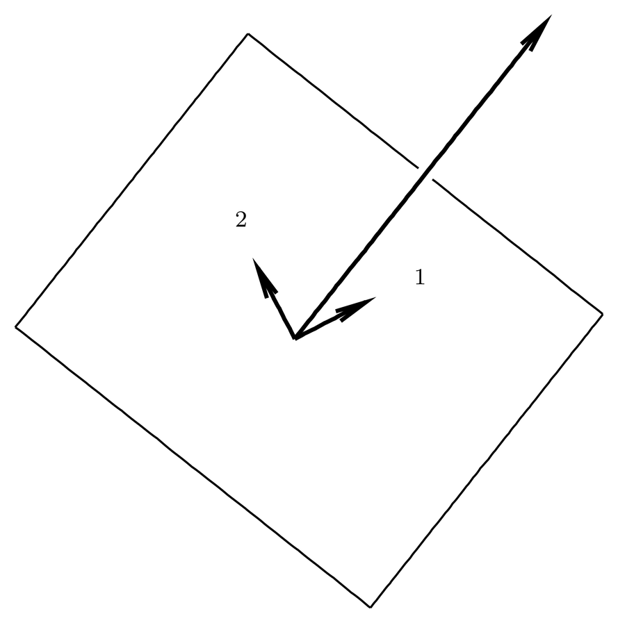
Figure 1:Polarization vectors and the transverse plane in -space.
We denote the polarization vectors by , where is the polarization index that labels the vectors. Polarization vectors must be allowed to be complex, in order to accommodate electromagnetic waves in which the phases of the different components differ. We choose them to be orthonormal in the sense of complex vectors, so they satisfy
They also satisfy
since they are transverse. Beyond these conditions, the polarization vectors are arbitrary, and, in particular, there is no necessary relation between polarization vectors for one value and another (in any case, the transverse planes are different for different values of ).
Taken with , the two polarization vectors form an orthonormal triad with a completeness relation (resolution of the identity) given by
so that an arbitrary vector can be expanded as
where
It is always possible to choose real polarization vectors, since is real. For example, if , then a pair of real polarization vectors is simply and . Real polarization vectors correspond to linearly polarized light, that is, a light wave for which the electric field vector at a fixed point of space traces out a line segment (going back and forth over it in each cycle). Complex polarization vectors can always be expanded as linear combinations of real polarization vectors. The relative phase (in the sense of complex numbers) of the two components of a complex polarization vector with respect to a real basis indicates the relative phase shift between the two components of the electric field. If this phase shift is , we have circularly polarized light, in which the electric field vector at a fixed point of space traces out a circle. Other phase shifts correspond to elliptically polarized light. The overall phase of a polarization vector is immaterial for determining the type of polarization; in this sense polarization vectors are like two-component spinors in quantum mechanics, for which the overall phase is nonphysical.
The Mode Expansion
Since the amplitude vectors are transverse, they can be expanded as a linear combination of the polarization vectors,
so that (53) becomes
We will regard this as a sum over the modes of the electromagnetic field, where each mode is specified by a value of and a polarization index . There are two modes for each lattice point in -space. We will often use the following abbreviation for the mode index,
for example,
We call the the mode amplitudes; they are complex numbers, one for each mode of the field. They satisfy the equations of motion
with the solution
Finally, the mode expansions of and are
The transformation (66) or its inverse (69) can be seen as another coordinate transformation, on top of (60),
a fairly trivial one, in fact, but it shows that knowledge of the mode amplitudes allows one to compute and and vice versa.
The Dynamical State of the Electromagnetic Field
In classical mechanics, the dynamical state of a system is the specification of enough information to determine the subsequent time evolution of that system. For example, in a mechanical system we can specify the positions and velocities (or momenta) of all the particles. In the case of the Schr"odinger equation, the dynamical state is specified by the wave function at a given time, , which constitutes a complete set of initial conditions since the Schr"odinger equation is first order in time. The wave equation (45), on the other hand, is second order in time, so a specification of the dynamical state of the system (the free field in Coulomb gauge) requires both and at a given time.
However, the coordinate transformation (60), given explicitly by (55) and (58), shows that the dynamical state of the electromagnetic field is equally well specified by the set of amplitude vectors . Or, with the subsequent coordinate transformation (74), it is specified by the set of mode amplitudes , one complex number for each mode of the field. These transformations can be regarded as coordinate transformations on the state space or phase space of the electromagnetic field. See Phase Space for this terminology in classical mechanics.
Although the transformation (60) was motivated by the plane wave solutions for the free field, you may notice that the transformation itself does not involve any equations of motion. It simply gives two alternative descriptions of the state of the field. It is true that for the free field in the description the equations of motion are the wave equation (45), while in the description or the equations of motion are (52) or (70). But these coordinate transformations can be used regardless of the equations of motion. Indeed, below we shall use these transformations in the case of the interacting field, for which the equations of motion are different from (45) or (52) or (70).
A Guess for the Canonical Coordinates
We return to our goal of finding a classical Hamiltonian description of the electromagnetic field, working for the moment with the case of the free field. To do this we require both a Hamiltonian and a proper definition of canonical coordinates, that is, a set of and coordinates in terms of which Hamilton’s classical equations of motion are equivalent to Maxwell’s equations. In this we guess the canonical coordinates.
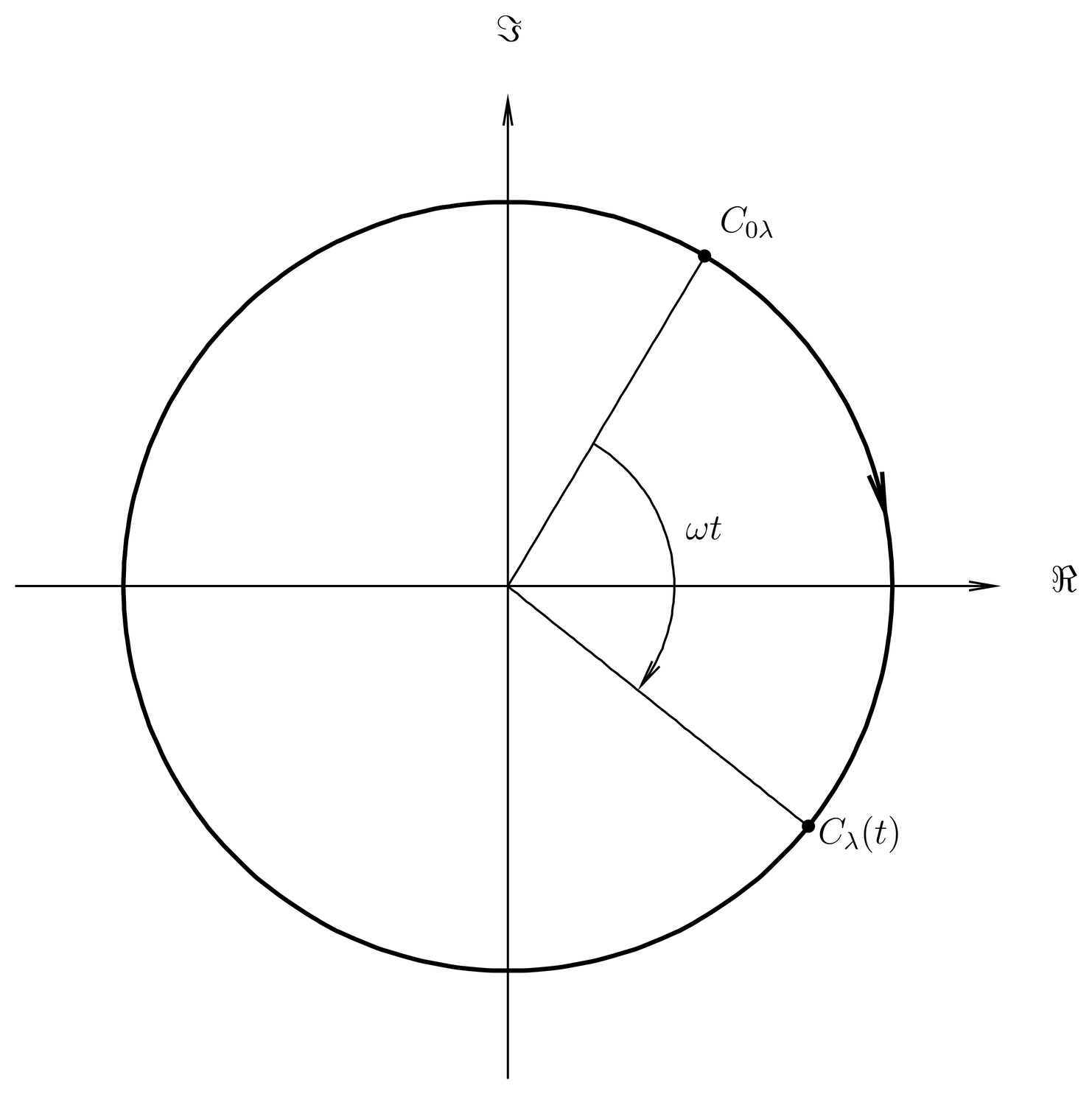
Figure 2:Evolution of mode amplitude in the complex plane.
For the free field, the mode amplitudes have the evolution given by (71). When viewed in the complex plane, the motion is circular in the clockwise direction, with frequency (the frequency of the light wave of the given mode). See Figure 2. This reminds us of the motion of a classical harmonic oscillator in the - phase plane (see Fig.~\figr\harmosc.1). This suggests that each mode of the free electromagnetic field can be described as a harmonic oscillator, and that the and the of the oscillator are proportional to the real and imaginary parts of , respectively.
To be more precise, the Hamiltonian for a mechanical harmonic oscillator is
whose orbit in phase space is an ellipse. But if we introduce the change of coordinates,
and then drop the primes, then in the new coordinates the Hamiltonian is more symmetrical between and ,
and the orbit in phase space is indeed now a circle. The motion is clockwise with frequency , just like the mode amplitude . The transformation (76) is an example of a canonical transformation in classical mechanics, in which phase space area is preserved (since the transformation squeezes in one direction and stretches in the other).
Now we introduce canonical coordinates for mode by writing,
where the constant is to be determined.
A Guess for the Free-Field Hamiltonian
In mechanical systems the Hamiltonian is the energy of the system, so we guess that the field Hamiltonian will be the energy of the field. That energy is
which we denote by in anticipation that this will prove to be the Hamiltonian. Since we are using periodic boundary conditions, we integrate only over the volume of the box.
To express in terms of the mode amplitudes, we write out Fourier series for and , using (73) for and differentiating (72) for . This gives
Let us look first at the integral of in the Hamiltonian (79). This is
There are four major terms in this integral; let us look at one of the cross terms, namely,
where we have carried out the spatial integration in the second equality, written and and done the -sum in the third equality, and then used (61) in the fourth equality. Thus we have evaluated one of the cross terms. By a similar calculation, we find that the other cross term in integral, as well as the two cross terms in the integral, all give the same answer as (86). As for the other terms (the -terms and the -terms), we find that these cancel when the electric and magnetic contributions are combined. Altogether, the Hamiltonian becomes
This tells us how to choose the constant in (78) to make the Hamiltonian come out as a sum of harmonic oscillators in the symmetrical form (77), one for each mode of the field. That is, we write
which defines and in terms of . Then The Hamiltonian becomes
Here we have written instead of to emphasize that depends on (so cannot be taken out of the sum). The field Hamiltonian is a sum of harmonic oscillators, one for each mode of the field.
Since there have been several guesses in the derivation of this Hamiltonian, we should now check to see that it really does give the correct equations of motion. But this is relatively easy. We have
which imply , which when used in the coordinate transformation (74) implies , which when used in the coordinate transformation (60), or, explicitly, (55), implies that satisfies the wave equation (45), which for the free field in Coulomb gauge implies Maxwell’s equations.
In classical mechanics, the number of independent ’s, or the number of pairs in the Hamiltonian, is called the number of degrees of freedom. We see that the electromagnetic field has one degree of freedom for each mode of the field (two per value). The total number of degrees of freedom is infinite.
The Field Interacting with Matter
We turn now to the case of the electromagnetic field interacting with matter. For this we must adopt some model of the matter. We will assume we have particles, with mass , charge , position and velocity , . We will use indices , , etc., to label the particles. The particles produce charge and current densities given by
Notice that is the field point, that is, the point of space where the charge or current density is measured, while is the position of the particle. We will henceforth maintain this notational distinction between field points () and particle positions (). Notice that acquires its time dependence because the particle positions depend on time; depends on time additionally through the particle velocity . These charge and current densities satisfy the continuity equation (5).
For the interacting field the equations of motion for the potentials in Coulomb gauge are (32). As noted in Field Equations in Coulomb Gauge, the scalar potential satisfies a non-retarded Poisson equation, with solution in terms of given by (34). With (91) for the charge density, the integral can be done, giving
This is a familiar formula from electrostatics, applied here, however, to electrodynamics, without retardation.
(34) or (93) shows that the scalar potential in Coulomb gauge is a function of the particle coordinates, that is, it is not an independent dynamical variable. If it were, it would satisfy some equations of evolution, and it would be necessary to specify initial conditions for to determine the values of at a later time. Instead, becomes completely known once the particle positions are known. This is in contrast to the transverse components of the vector potential, which are true dynamical degrees of freedom of the field, and which, as we have seen in the case of the free field, are associated with a set of independent ’s and ’s.
Another way to express in terms of the matter degrees of freedom is to Fourier transform the Poisson equation, (32), which gives , or
We will assume the total charge in the box is zero, so at and there is no problem with in (94).
Of the four components of the 4-vector potential , one () is a function of the matter degrees of freedom, one (the longitudinal component of ) vanishes, and two (the transverse components of ) are true dynamical variables of the field. This is how it works in Coulomb gauge. In other gauges the results are similar; the electromagnetic field has only two true degrees of freedom for each value of .
The equation of motion for interacting with matter is (33). Since the left-hand side of this equation is purely transverse, the right-hand side must be purely transverse also. But the term is purely longitudinal, so we suspect this must cancel out the longitudinal part of the current . To check that this is true, we transform (33) to -space, obtaining
and dot with to obtain
The longitudinal component of the current can be expressed in terms of the charge density by Fourier transforming the continuity equation (5),
or . The continuity equation constrains the longitudinal component of the current, but imposes no constraints on the transverse part. Also, from (94) we have . When these are used in (96), the two terms on the right-hand side cancel, verifying our suspicions.
Thus, the continuity equation and the Poisson equation imply that the right-hand side of (33) is purely transverse, and we can write
In Coulomb gauge, the vector potential, which is purely transverse, is driven by the transverse components of the current. Since was described by harmonic oscillators in the case of the free field, we suspect that it will be described by driven harmonic oscillators in the case of the interacting field, where the driving terms depend on the matter degrees of freedom. This will result in a transfer of energy between the matter and field, that is, it will result in the emission and absorption of radiation.
Mode Amplitude Equations of Motion for the Interacting Field
To see these driven harmonic oscillators explicitly, we will define the amplitude vectors in terms of by (53) or their inverse (58), effectively borrowing the coordinate transformation (60) from the free-field case for use in the case of the interacting field. The equation of motion for , however, is now the driven wave equation (98), not the free wave equation. Thus we must find the new equations of motion for the amplitude vectors , something to replace (52).
To do this we first project out the transverse components of (95), obtaining
after multiplying through by . Next we compute the quantity , which vanishes for the free field. Using (58), we have
But by (99), this becomes
This is the equation of motion for the amplitude vectors for the interacting field that replaces (52) for the free field.
Next we project out the components of along the polarization vectors as in (69), so that
and similarly for the components of . Thus we obtain the equations for the mode amplitudes for the interacting field,
which replaces (70) for the free field.
The method we are following here, of borrowing definitions made in the case of the free field and using them (with modified equations of motion) for the interacting field, is known in the theory of differential equations as Lagrange’s method of variation of parameters. It is often useful for driven linear systems, precisely the type of system we are dealing with here.
The Hamiltonian for the Matter-Field System
As in the case of the free field, we guess that the Hamiltonian for the combined matter-field system will be the total energy of that system. This energy consists of two parts, a matter (kinetic) energy and a field energy, so we write
At this point we are using the nonrelativistic expression for the kinetic energy of the particles, and, in fact, this is the first point where we have assumed that the particles are nonrelativistic. We could create a relativistically covariant classical model by using the relativistic expression for the kinetic energy of the particles, but that would lead to difficulties upon quantization since so far we only know how to handle nonrelativistic matter in quantum mechanics. We will deal with relativistic quantum mechanics later in the course, but for now we must restrain our ambitions.
You may wonder where the potential energy of the matter is in (105). As we shall see, the potential energy is hiding in the field energy. Without knowing this, however, we can check to see that the total energy, as defined by (105), is actually a constant of motion. To do that we must call on Maxwell’s equations (2) and (4) for the field, and the nonrelativistic Newton-Lorentz equations of motion for the matter,
When is expanded out by the chain rule, applied to (105), and the equations of motion are used, one finds . The quantity defined by (105) is an exact constant of motion (the total energy) of the combined system of matter plus field.
The expression for the field energy in (105) is the same as the one we used in the case of the free field, but now now contains both a longitudinal and transverse part, see (35). Thus the electric field energy is
But the cross terms in the dot product cancel when integrated over the box, due to the Parseval identity (see (31) or (41)). Thus, the electric field energy decomposes into a longitudinal part and a transverse part.
As for the longitudinal part, it is
where we integrate by parts in the second equality, use the Poisson equation (32) in the third, the expression (91) for in the fourth, which allows the integral to be done, and the expression (93) for in the fifth. We see that the longitudinal field energy is otherwise the nonretarded Coulomb potential energy of the collection of point particles. The factor of compensates for the double counting of particle pairs.
Unfortunately, this sum contains the diagonal terms , which are infinite. These terms represent the infinite self-energy of the point particles, which as mentioned previously is a fundamental difficulty in classical electrodynamics. We will simply discard these infinite diagonal terms, and hope that the resulting theory makes sense. (In fact, it does, but only to lowest order in perturbation theory.)
As for the transverse electric contribution to the field energy, can be represented as a Fourier series over modes by calling on (73), which leads to the same series in (80) that was used in the case of the free field (in that case, the transverse electric field was the total electric field). Similarly, the Fourier series for the magnetic field is given by (81), which was used in the case of the free field. Thus the transverse electric and magnetic contributions to the energy, when expressed in terms of mode amplitudes, lead to the same sum over modes, (87), as in the case of the free field.
Next we guess that the correct definition of and for the interacting field is the same one used for the free field, (88), since if we drive a harmonic oscillator we do not change its or , we just change the equations of motion. Thus the transverse field energy is given by the same sum over harmonic oscillators, (89), that we found in the case of the free field. Thus we have
As for the kinetic energy of the matter in (105), it is expressed in terms of the velocities of the particles. But Hamiltonians are normally expressed in terms of momenta, not velocities. We guess that the correct definition of the momenta of the particles is the one that is usually used in the classical dynamics of particles interacting with electromagnetic fields,
that is, in situations where one is studying the motion of particles in given (external) fields and not attempting to include the dynamics of the field, as we are here. With this substitution, we can write the total Hamiltonian for the matter-field system as
where
and
Again, we have made several guesses and must check that this Hamiltonian gives the correct equations of motion, according to Hamilton’s equations. The equations of motion are the Newton-Lorentz equations (106) for the matter, and (104) for the mode amplitudes, which, as shown in Mode Amplitude Equations of Motion for the Interacting Field, are equivalent to the driven wave equation (98) for , which is equivalent to the full Maxwell equations. This check will be left as an exercise.
Exactly Conserved Quantities
The combined matter field system has several exactly conserved quantities, in addition to the energy or Hamiltonian, given by (105). These can be obtained in a systematic manner by writing down the Lagrangian for the matter-field system and then applying Noether’s theorem, which is a general relation between symmetries and invariants in Lagrangian mechanics. The matter-field Lagrangian is invariant under several space-time symmetries, including time translations, spatial translations, and rotations. The conserved quantity associated with time translations is the energy or Hamiltonian, which we have already discussed. The conserved quantity associated with spatial translations is the momentum, given by
This is the expression for the total momentum of the matter-field system, using our nonrelativistic model for the matter. One can show explicitly that , by appealing to the equations of motion. The field contribution is proportional to the integral of the Poynting vector , which is the energy flux of the electromagnetic field. This however is proportional to the momentum density, .
Notice that the matter contribution to the momentum is just the kinetic momentum. You may wonder where the extra term is, which is added to the kinetic momentum to get the canonical momentum , as in (111). The answer is that in Coulomb gauge, this term comes from the longitudinal contribution to the field momentum, that is, it is the integral of . This correction term, taking us from the kinetic to the canonical momentum, is necessary for a Hamiltonian description of charged particles interacting with fields, but it is somewhat mysterious when the fields are just considered given. But by including the field as a part of the dynamical system, we see that this contribution is just part of the field momentum. The total momentum of the matter-plus-field system is a rather simple expression.
The energy and momentum constants of motion can also be obtained by working with the stress-energy tensor for the combined matter-plus-field system. This approach is most elegant in a relativistic treatment, in which the four-divergence of the stress energy tensor vanishes. This leads to four continuity equations, one for energy and three for the components of momentum. When these are integrated over all space, the energy and momentum constants of motion emerge. The constants we have quoted above for and are the limits of the relativistic constants when the velocities of the material particles are low.
The invariance of the classical Lagrangian under rotations leads to a conservation law for angular momentum. The total angular momentum of the matter-plus-field system is
where (the total angular momentum) is not to be confused with the current.
These exactly conserved quantities for the combined matter-plus-field system are the only ones that exist for that system. We have given a somewhat abbreviated discussion of them because most of the details belong in a course on classical electromagnetism. These classical conserved quantities will be of use to us later when we quantize the electromagnetic field.
Normal Variables
Finally, we make one further cosmetic change in preparation for quantization. We define new variables ,
which are obviously just classical analogs of annihilation and creation operators in quantum mechanics. We call these variables normal variables. The normal variables are related to the by
Expressing the vector potential and field Hamiltonian in terms of the normal variables, we have
and
The fields and can also be expressed in terms of normal variables,
and
Problems
Problem 1.
Retardation in the Coulomb gauge. A particle with charge is located at the origin of the coordinates. In the interval 0 to the particle is displaced from the origin to along a path (). Let be a point distant from the origin at which we make measurements of the field. Assume . Also assume , which means that an observer at position cannot know that the particle has moved, since the light signal from the particle cannot have reached the observer in time . The purpose of this exercise is to prove, starting with Maxwell’s equations, that the instantaneous variations of the longitudinal electric field created by charge at are exactly compensated by the instantaneous component of the transverse electric field produced by the displacement of the particle.
(a) Calculate, as a function of , the electric field at point and time from charge . Show that can be written,
where is given by a power series in . Show that the lowest order term of this expansion can be expressed as a function of and of the transverse -function, .
(b) Find the current associated with the motion of the particle. Express the transverse current at the point of observation as a function of and the transverse -function . Explain why to the lowest order in , one can replace by . Write the Maxwell equation giving in terms of and . Begin by ignoring the contribution of to . Integrate the equation between 0 and . Show that the transverse electric field produced by compensates exactly (to lowest order in ) the field found in part (a). The small parameter here is , not ; the particle motion could be fast (relativistic).
(c) By eliminating the electric field from Maxwell’s equations, find the equation of motion for the magnetic field . Justify the approximation made above of neglecting the contribution of to over short periods ().
Problem 2.
Several guesses were made in deriving the classical Hamiltonian for the matter-field system, Eqs.~(\eqr\cn.96)--(\eqr\cn.98), so we should check the answer to see that it give the correct equations of motion. This Hamiltonian is a function of the and the , which are the ’s and ’s of the system. All dynamical variables are considered to be functions of the ’s and ’s. For example, , and are defined by Eqs.~(\eqr\cn.103), (\eqr\cn.105) and (\eqr\cn.106), in which the Fourier series contain and , which in turn are defined in terms of and by Eq.~(\eqr\cn.101). For the purposes of this problem, it will be better to indicate explicitly that the fields depend not only on the field point but also on the and . For example, we will write for the vector potential evaluated at a field point .
Please note the difference between , an arbitrary point of space at which a field may be evaluated, and , the position of particle . The field point is not a dynamical variable; it does not have an equation of evolution. The point is a dynamical variable; it does have an equation of motion.
The quantity is classical, in spite of the . We could have written in terms of the mode amplitude , defined by (103), but , which is proportional to , is more convenient since it carries over to the annihilation operator in quantum mechanics.
(a) Use the chain rule to show that Hamilton’s classical equations for and are equivalent to
which are more convenient for the following work. Notice that these equations are complex conjugates of each other.
(b) Now use Hamilton’s equations for to obtain
(c) What we mean by is the time derivative of the field , evaluated at some field point , holding fixed. We also call this . The time evolution is due to the time dependence of the and , upon which depends. With this understanding, we have
where we have shown explicitly that depends on the and . Show that Hamilton’s equations imply
This is equivalent to (73), with the coefficients replaced by according to (119). Hint: Notice the resolution of identity, (63), which allows you to do the polarization () sum.
(d) Now show that
where is the total electric field, longitudinal plus transverse. Notice that the time derivative of must be interpreted as
since the field is evaluated at the particle position, and the particle position is moving.
(e) Finally show that
This equation is equivalent to Maxwell’s equations.
Problem 3.
Equation~(\eqr\cn.99) gives the total momentum of the matter-field system. Using Newton’s laws for the particles and Maxwell’s equations for the field, show that . Hint: You can integrate by parts, throwing away boundary terms, assuming that all fields die off at spatial infinity. If you are astute you will see the appearance of the stress-energy tensor in this calculation.