01. The Mathematical Formalism of Quantum Mechanics
Introduction
The prerequisites for Physics 221A include a full year of undergraduate quantum mechanics. In this semester we will survey that material, organize it in a more logical and coherent way than the first time you saw it, and pay special attention to fundamental principles. We will also present some new material. Physics 221B will largely consist of new material.
We begin by presenting some of the mathematical formalism of quantum mechanics. We will introduce more mathematics later in the course as needed, but for now we will concentrate on the linear algebra of spaces of wave functions, which are called Hilbert spaces. These notes gather together and summarize most of what you will need to know of this subject, so we can proceed with other matters. In the next set of notes we will turn to the physical postulates of quantum mechanics, which allow us to connect experimental results with the mathematics presented here.
Introductory courses on linear algebra are usually limited to finite-dimensional, real vector spaces. Making the vector spaces complex is a small change, but making them infinite-dimensional is a big step if one wishes to be rigorous. We will make no attempt to be rigorous in the following---to do so would require more than one course in mathematics and leave no time for the physics. Instead, we will follow the usual procedure in physics courses when encountering new mathematics, which is to proceed by example and analogy, attempting to gain an intuitive understanding for some of the main ideas without going into technical proofs. Specifically, in dealing with Hilbert spaces we will try to apply what we know about finite-dimensional vector spaces to the infinite-dimensional case, often using finite-dimensional intuition in infinite dimensions, and we will try to learn where things are different in infinite dimensions and where one must be careful. Fortunately, it is one of the consequences of the mathematical definition of a Hilbert space that many of its properties are the obvious generalizations of those that hold in finite dimensions, so much of finite-dimensional intuition does carry over. We will use what we know about spaces of wave functions (an example of a Hilbert space) to gain some intuition about where this is not so.
Hilbert Spaces
Let us consider a wave function for a one-dimensional quantum mechanical problem. In practice it is common to require to be normalized, but for the purpose of the following discussion we will require only that it be normalizable, that is, that
(which means that the integral is finite; usually when we write an integral without limits like the one above, we mean that the limits are to , or over all of space if the integral is multidimensional). Wave functions that are not normalizable cannot represent physically realizable states, because the probability of finding a real particle somewhere in space must be unity. Nevertheless, wave functions that are not normalizable, such as the free particle energy eigenfunctions , are definitely useful for some purposes, and we will have to say something about them later. For now, however, we will stick to normalizable wave functions.
Mathematically speaking, the space of complex functions that are normalizable (or square integrable) in the sense of (1) constitutes a complex vector space. This is because if is square-integrable, then so is , where is any complex number, and if and are square-integrable, then so is . Moreover, the space is infinite-dimensional (see Mathematical Notes). This vector space is an example of a Hilbert space; in general, a Hilbert space is a complex, inner product vector space (a vector space upon which an inner or scalar product is defined) with certain additional properties that will not concern us in this course (see Mathematical Notes). Often the term “Hilbert space” is defined to be an infinite-dimensional space, but in this course we will refer to any of the vector spaces of wave functions that occur in quantum mechanics as Hilbert spaces, even when finite-dimensional.
As you know, given a normalized wave function in configuration space, is the probability density for making measurements of position on an ensemble of systems. The wave function is connected physically with position measurements. (See Constrained Systems, Configuration Space, and Generalized Coordinates for the definition of “configuration space.”)
Given in configuration space, one can compute the corresponding wave function in momentum space, by a version of the Fourier transform:
The Fourier transform is linear and invertible (via the inverse Fourier transform), so it provides a one-to-one, linear map between the space of wave functions and that of . Moreover, according to the Parseval identity, the norm of in configuration space and the norm of in momentum space are equal,
so if we consider the Hilbert space of normalizable wave functions in configuration space, then the set of corresponding momentum space wave functions also forms a Hilbert space. (The “norm” of a wave function is the square root of the quantity shown in (3); it is like the length of a vector.)
The momentum space wave function is connected with the measurement of momentum, in particular, if is normalized then is the probability density for momentum measurements on an ensemble of systems. The Parseval identity expresses the equality of the total probability for measurements of either position or momentum.
Likewise, let be an orthonormal set of energy eigenfunctions, for some Hamiltonian . An arbitrary wave function can be expanded as a linear combination of the functions , that is, we can write
where the expansion coefficients are given by
(4) can be regarded as a linear transformation taking us from the sequence of coefficients to the wave function , while (5) goes the other way.
The sequence of coefficients uniquely characterizes the state of the system, and we can think of it as the “wave function in energy space.” Notice that if the sequence is normalized, , then the probability of making a measurement of energy is . Also, the norm of the original wave function can be expressed in terms of the expansion coefficients by
which is finite if belongs to Hilbert space. This is another expression of conservation of probability. Mathematically speaking, the set of sequences of complex numbers of finite norm is yet another example of a Hilbert space.
Thus, we have three Hilbert spaces, the two spaces of wave functions, and , and the space of sequences , all assumed to be normalizable. These Hilbert spaces are isomorphic, in the sense that the vectors of each space are related to one another by invertible, norm-preserving linear transformations, so they all contain the same information. (See Mathematical Notes for some mathematical points regarding Hilbert spaces of wave functions.) Therefore none of these spaces can be taken as more fundamental than the other; any calculation that can be carried out in one space (or in one representation, as we will say), can be carried out in another.
Psychologically, there is a tendency to think of wave functions on configuration space as fundamental, probably because we are used to thinking of fields such as electric fields defined over physical space. This is also the bias imposed on us by our first courses in quantum mechanics, as well as the historical development of the subject. Also, we live in physical space, not momentum space. But the Schr"odinger wave function is not really defined over physical space, rather it is defined over configuration space, which is the same only in the case of a single particle (see Constrained Systems, Configuration Space, and Generalized Coordinates). Furthermore, completely apart from the mathematical equivalence of the different Hilbert spaces discussed above, the physical postulates of quantum mechanics show that the different wave functions discussed above correspond to the measurement of different sets of physical observables. They also show that there is a kind of democracy among the different physical observables one can choose to measure, as long as the set of observables is compatible and complete in a sense we will discuss later.
Finally, even if we do have a single particle moving in three dimensions so the wave function can be thought of as a field over physical space, the physical measurement of is very different from the measurement of a classical field such as the electric field or the pressure of a fluid. We have thermometers that can measure the temperature at a point, we have pressure gauges, and it is possible to measure electric and magnetic fields at points of space. But there is no such thing as a “-meter” for measuring the wave function . Later we will consider how one can obtain from measurements, but the process involves several subtleties. (In particular, it requires one to understand the difference between a pure and a mixed state; only pure states have wave functions.) It is a very different business than the measurement of a classical field. See Prob. Paragraph.
In summary, it is probably best to think of the different wave functions as equivalent descriptions of the same physical reality, none of which is more fundamental than the other. This leads to the concept of the state space of a quantum mechanical system as an abstract vector space in which the state vector lies, while the various wave functions are the expansion coefficients of this state vector with respect to some basis. Different bases give different wave functions, but the state vector is the same.
This was not the point of view in the early days of quantum mechanics, when was seen as a complex-valued field on physical space, and before it was completely clear what the wave function of multiparticle systems should be. We will return to this earlier point of view when we take up the Dirac equation and field theory, but that reconsideration will not change the basic concept of the state space for the quantum mechanical system, a complex vector space in which the state vector lies.
Thus, the mathematical formalism of quantum mechanics exhibits a kind of form invariance or covariance with respect to the set of observables one chooses to represent the states of a system. This view of quantum mechanics, and the transformation theory connected with changes of representation, was worked out in the early days of the quantum theory, notably by Dirac, Born, Jordan, von Neumann and others.
Dirac Ket Notation
Since none of the three Hilbert spaces has any claim over the other, it is preferable to use a notation that does not prejudice the choice among them. This is what the Dirac notation does. In the Dirac notation, a state of a system is represented by a so-called ket vector, denoted by , which stands for any of the three wave functions discussed above, , , or , assuming that they are related by the transformations (2) and (5). It is customary to put a symbol into the ket to identify the state, to write, for example, [although the choice of the letter seems to point to something special about the configuration space wave function , which there is not]. Some people think of a ket as simply another notation for a wave function on configuration space, and I have even seen some authors write equations like
But our point of view will be that the space of kets is yet another Hilbert space, an abstract space that is isomorphic to but distinct from any of the concrete Hilbert spaces of wave functions discussed above. Thus, we will never use equations like (7). I think this approach is appropriate in view of the physical postulates of quantum mechanics, which show how one can construct a Hilbert space out of the results of physical measurements. There is no need to start with wave functions. Therefore we will now put wave functions aside, and discuss the mathematical properties of ket spaces. Later, in 04. Spatial Degrees of Freedom, we will return to wave functions, in effect deriving them from the ket formalism. In this set of notes, we use wave functions only for the purpose of illustrating some general features of Hilbert spaces, calling on your experience with them in a previous course in quantum mechanics.
Kets, Ket Spaces and Rays
Kets and ket spaces arise out of the physical postulates of quantum mechanics, which we will discuss in 02. The Postulates of Quantum Mechanics. For now we will just say enough to get started.
A basic postulate of quantum mechanics is that a given physical system is associated with a certain complex vector space, which we will denote by . The physical principles by which this vector space is constructed will be discussed later, but for now we simply note that the properties of this space such as its dimensionality are determined by the physics of the system under consideration. For some systems, is finite-dimensional (notably spin systems), while for others it is infinite-dimensional. The vectors of the space are called kets, and they are denoted in the Dirac notation by , as discussed above. Since is a complex vector space, the multiplication of kets by complex numbers and the addition of kets is defined. The product of a complex number and a ket can be written in either order,
In addition, there exist physical principles that allow us to associate a definite (pure) state of a physical system with a ray in . We will say more about this association later, when we will define what we mean by a pure state of a physical system, but for now we simply note that a ray in is a 1-dimensional vector subspace of , that is, it consists of kets related to some nonzero ket by a complex multiplicative factor, that is,
for some complex number . The kets in the ray differ from one another only by normalization and overall phase, which have no physical significance; thus, we say that a (pure) physical state corresponds to the ray (not to any particular ket in the ray).
The Dual Space and Bras
You are probably familiar with the fact that kets correspond to wave functions , while bras correspond to complex conjugated wave functions . But if we are doing without wave functions until we can properly derive them, how do we describe bras and the complex conjugation of kets? The answer is the dual correspondence.
Also, it would appear that is just another wave function, so it should belong to the same space of wave functions as . But it turns out that there is great advantage in regarding kets and bras as belonging to two different spaces. Kets belong to the space , while bras belong to the so-called dual space, denoted .
If is any (complex) vector space, then the dual space, denoted , is the space of complex-valued, linear operators that act on . In the Dirac notation, such operators are called bras, and are denoted . (In mathematics, they are called forms, covectors or dual vectors.) As with kets, it is customary to insert some symbol to identify a bra and distinguish it from other bras, such as . In mathematical language, we write
which means that maps a ket into a complex number. To be a bra, the map must be linear. If is a ket, then the complex number that results by letting act on it can be written . Usually we drop the parentheses write the complex number simply as , but if we wish to emphasize the interpretation of the bra as an operator acting on kets we will keep the parentheses.
Since the map is required to be linear, we have
A bra, as a linear operator acting on kets, is not to be confused with the familiar linear operators used in quantum mechanics, such as the Hamiltonian operator, which also act on kets. The distinction is that a bra is a complex-valued operator, whereas the Hamiltonian and other such operators are ket-valued operators.
It is easy to see how to define the product of a bra with a complex scalar, and the sum of two bras; we simply set
and
Therefore the set of all bras acting on a given ket space forms a vector space in its own right, which by definition is the dual space . It is easy to show that if is finite-dimensional, then is also, and has the same dimension. If is infinite-dimensional, then the dual space is also infinite-dimensional.
What we have said so far allows us to talk about bras, but not to convert a ket into a bra (the analog of the complex conjugation of wave functions). To do that we need to introduce the metric or scalar product on our ket space. In real, Euclidean vector spaces the metric is what allows us to measure distances, and from that, angles. This is an analogy to keep in mind while thinking about the metric in (complex) Hilbert spaces, because it provides useful geometrical interpretations.
The Scalar Product and Dual Correspondence
We postulate the existence of a metric or scalar product on , which is a function
with certain properties. This notation means that is a function that takes two kets and produces a complex number; for example, we will write for the complex number that results upon letting act on kets and . The postulated properties of are the following. First, is linear in its second operand and antilinear in its first operand. Explicitly, this means
(An antilinear function requires us to take the complex conjugate of the coefficients when evaluating it on linear combinations of vectors.) Next, is symmetric or Hermitian, which means
Third, is positive definite, which means
for all , with equality holding if and only if . Note that by property (17), the left hand side of (18) is necessarily real.
Next, given the metric , we can define the dual correspondence, which is a mapping that converts kets into bras. It is the map which in wave function language amounts to taking the complex conjuate of a wave function. We will denote the dual correspondence by ; it is the map
If is a ket, then we will denote the bra corresponding to it under the dual correspondence by , with the same identifying symbol. We define the bra in terms of its action on an arbitrary ket ; the definition is
The idea is that in the scalar product, we regard the first argument as fixed and the second as variable, which gives us a complex valued function of kets, which according to (15) is linear. Thus, the function is a bra. By way of notation, we will denote the bra resulting from a given ket under the dual correspondence by a dagger, so that if
then we will write
We will say that is the Hermitian conjugate of . We note that since the scalar product is antilinear in its first operand, the dual correspondence is antilinear, that is,
If is finite-dimensional, then it is easy to prove that the dual correspondence is one-to-one and onto, so that every bra is in fact the Hermitian conjugate of some ket. This follows from the postulated properties of the metric. In infinite-dimensional spaces, this is true only if certain restrictions are placed on the bra space. We will ignore such technicalities, and proceed as if the dual correspondence is always one-to-one and onto (which, with the right understandings, it is for a Hilbert space). This means that every bra is the dagger of some unique ket, so the dual correspondence has an inverse. We will denote the inverse with the same dagger notation, so that
and so that
We now simplify the notation for the scalar product by dropping the parentheses on the left hand side of (20). That is, we write
With this notational change, we can rewrite properties (17) and (18) of the metric as
and
for all , with equality if and only if . The complex number is sometimes called the inner product or scalar product of and . Using the notation shown in (26), we can henceforth dispense with the -notation when talking about scalar products.
The Schwarz Inequality
We can now prove an important theorem, namely the Schwarz inequality. We are interested in this inequality for complex vector spaces, but it is also true in real vector spaces with a positive definite inner product, that is, in Euclidean spaces. There it is equivalent to the geometrical fact that the shortest distance between two points is a straight line. The Schwarz inequality is important in quantum mechanics because it is used to prove the Heisenberg uncertainty relations.
The Schwarz inequality says that
for all and , with equality if and only if and are linearly dependent, that is, if they lie in the same ray. To prove the theorem, we set
where is a complex number, and we use (28) to write,
This is true for all kets and , and all complex numbers . Since the Schwarz inequality is obviously true if , we consider the case , and we set
so that (31) becomes
which is equivalent to (29). Finally, it is easy to show that (33) becomes an equality if for any complex number , and conversely, if (33) is an equality, then , which implies , or . Therefore the equality holds in (29) if and only if and are linearly dependent.
Operators
Next we discuss operators. Usually in quantum mechanics we use only linear or antilinear operators. A linear operator and an antilinear operator are both mappings from the ket space into itself,
but they have different properties when acting on linear combinations of kets. In particular, we have
The only antilinear operator of interest in nonrelativistic quantum mechanics is the time-reversal operator, which we will discuss in 22. Time Reversal. For now we ignore antilinear operators, and concentrate exclusively on linear operators.
Linear operators themselves can be multiplied by complex numbers and added, so they form a complex vector space in their own right. Linear operators can also be multiplied with one another; the product means, apply first, then (to some ket). The multiplication is associative,
for any linear operators , , , but it is not commutative, that is
in general. The lack of commutativity of two linear operators and is measured by their commutator, defined by
For reference, we also define the anticommutator,
We use the same curly bracket notation for the anticommutator as for the Poisson bracket in classical mechanics (see The Poisson Bracket). It will usually be clear from context which is intended.
A linear operator may possess an inverse, ; if it exists, it satisfies
where the identity operator is simply denoted by 1. In finite-dimensional spaces, if exists, then it is both a right- and a left-inverse; but in infinite dimensional spaces, some operators may possess a right-inverse but not a left-inverse, or vice versa. When all indicated inverses exist, we have
A more careful treatment of the subject of operator inverses in infinite-dimensional spaces must deal with domains of definition, boundedness and other matters. We may wish to gloss over these in a first course in practical quantum mechanics.
Rules for Commutators
The commutator obeys the following properties, which are trivial consequences of the definition (39). In the following, capital letters are linear operators and lower case letters are complex numbers. First, the commutator is linear in both operands,
it is antisymmetric,
and it obeys the Jacobi identity,
Any bracket operation defined on any vector space (not just spaces of linear operators) that satisfies properties (43)--(45) qualifies that vector space as a Lie algebra.
In addition, the commutator satisfies the following properties, sometimes referred to as the derivation property or Leibnitz rule:
Calculations in quantum mechanics often require one to reduce complicated commutators into simpler ones that are known. Rules (46) are especially useful for this purpose. It is interesting that properties (43)--(46) are also valid for the Poisson bracket in classical mechanics [except that the ordering of the factors in (46), which must be respected in quantum mechanics, is immaterial in classical mechanics]. See The Poisson Bracket.
The Action of Operators on Bras
The operators we have introduced begin life as operators that act on kets, mapping them into other kets; but the definition of these operators is easily extended to allow them to act on bras, whereupon they produce other bras. If is a bra and an operator, we denote the action of on by , with the bra to the left. That is, we think of as acting on kets to the right, but on bras to the left. The definition of is as follows. Since is supposed to be a new bra, it is specified by its action on an arbitrary ket, say, ; the definition is given by writing
Since by this definition the ordering of the parentheses is immaterial, it is customary to drop them, and to write simply
Thus, we can think of as acting either to the left or the right in the “matrix element” .
The Outer Product
If and are kets, then we can define a linear operator denoted by , whose action on an arbitrary ket is given by
where the right-hand side is the product of the complex number times the ket . The action of on bras is given by
This is not the definition of , which is given by (49), rather it is a simple consequence of that definition. Its proof will be left as an exercise. The operator can be viewed as the tensor product of the ket with the bra ; this kind of product is similar to the dyadic product used in ordinary vector or tensor analysis. The operator is called the outer product of and .
Bases and Orthonormal Bases; Resolutions of the Identity
As in any vector space, a basis is a set of linearly independent vectors that span the entire space, and the number of such vectors is the dimension of the space. This is a familiar concept in finite dimensions. In an infinite-dimensional space, we obviously need an infinite number of basis vectors, but is the basis countably or uncountably infinite? That is, can we label the basis vectors with a discrete index, or do we need continuous indices as well? As it turns out, it is one the mathematical properties of Hilbert spaces that they always possess a countable basis, that is, a set of linearly independent, normalizable vectors that span the space and can be indexed , or by some other such discrete indexing scheme. This does not mean that every basis we encounter will be labeled by a discrete index, only that such bases always exist. In fact, in practice in quantum mechanics we frequently encounter “bases” with continuous indices as well, but the basis vectors of the continuum are not normalizable and do not belong to Hilbert space. We will say more about these kinds of bases later, and for now proceed with the case of discrete bases, consisting of normalizable vectors. As an example, you may think of the harmonic oscillator wave functions in one-dimensional quantum mechanics, which are normalizable, belong to Hilbert space, and form a discrete, complete set.
Let us denote a discrete basis in a ket space by . We say the basis is orthonormal if
We usually use orthonormal bases in quantum mechanics, but non-orthonormal bases are useful sometimes as well (if more difficult to work with). In any basis, an arbitrary ket can be represented as a linear combination of the basis vectors,
and if the basis is orthonormal, the expansion coefficients are given by
Substituting this into (52), we have
or, since is arbitrary,
where 1 is the identity operator. This is the resolution of the identity associated with the orthonormal basis .
Resolutions of the identity associated with bases with continuous indices will be discussed below.
Hermitian Conjugation
We have already defined Hermitian conjugation (denoted by the dagger ) of bras and kets. We now define Hermitian conjugation of operators. If is a linear operator, then is another linear operator, defined by its action on an arbitrary ket by
We should note that is an antilinear function of (because of the dual correspondence), but when we do the (second) Hermitian conjugation indicated on the right hand side of (56), the result is a linear function of . Thus, is a linear operator.
There are a number of immediate consequences of this definition, which we list here. The proofs are left as simple exercises.
We have now defined the action of the Hermitian conjugate operation on kets, bras, and operators. It is convenient also to define the action of the Hermitian conjugate on complex numbers as being identical with ordinary complex conjugation. With this understanding, we can state a general rule, which is illustrated in several various ways in the results above, which says that the Hermitian conjugate of a product of objects (kets, bras, operators, complex numbers) is given by reversing the order of the objects and replacing each by its Hermitian conjugate. The products involved can be either ordinary multiplication by scalars, operator products, or inner or outer (tensor) products. We only require that the original product be meaningful.
Hermitian, Anti-Hermitian and Unitary Operators
We say that an operator is Hermitian if it is equal to its own Hermitian conjugate,
An equivalent definition is
for all kets and . Similarly, an operator is said to be anti-Hermitian if it satisfies
An arbitrary operator is in general neither Hermitian nor anti-Hermitian, but can always be uniquely decomposed into a sum of a Hermitian and an anti-Hermitian operator:
If is Hermitian, then the matrix element is necessarily real, for all choices of , in accordance with (57). We say that a Hermitian operator is positive definite if it satisfies
for all nonzero kets . Similarly, we say that is nonnegative definite if
for all kets .
We have not discussed eigenvalues yet, but a positive definite, Hermitian operator is one whose eigenvalues are all positive, while a nonnegative definite, Hermitian operator is one whose eigenvalues are all nonnegative.
A simple but important theorem is the following:
The (trivial) proof is left as an exercise.
An operator is unitary if
so that
The product of two unitary operators is always unitary.
Eigenvalues and Eigenkets; the Spectrum of an Operator
If is an operator acting on and there exists a nonzero ket and complex number such that
then we say that is an eigenket of and is a (right) eigenvalue. Similarly, if there exists a nonzero bra and a complex number such that
then we say that is an eigenbra of and is a (left) eigenvalue. In finite dimensions, every right eigenvalue is also a left eigenvalue, but in infinite dimensions this need not be true.
We define the spectrum of an operator as the set of its eigenvalues, seen as a subset of the complex plane. (If necessary, we can distinguish between a left and right spectrum.) In finite dimensions, this is a set of discrete points in the complex plane.
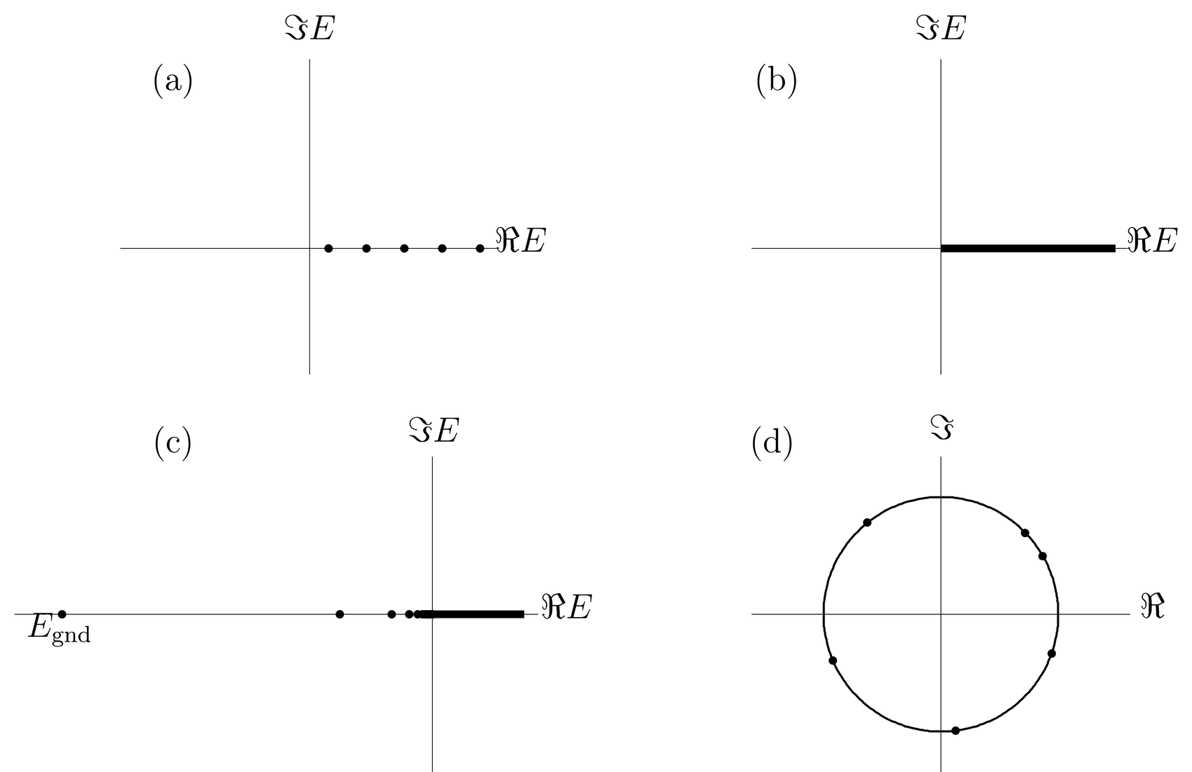
Figure 1:Examples of spectra of operators. Part (a), the harmonic oscillator; part (b), the free particle; part (c), the hydrogen atom; part (d), a finite-dimensional unitary operator.
Some examples of the spectra of familiar operators in quantum mechanics are illustrated in Figure 1. In part (a) of the figure we have the spectrum of the harmonic oscillator, whose eigenvalues are shown as spots on the real energy axis. This is an example of a discrete spectrum. Only real energies are physically meaningful, but we show the whole complex energy plane because in general eigenvalues of operators are complex. (We will see complex energies play a role in scattering and resonance theory later in the course.) In part (b) we have the spectrum of the free particle Hamiltonian . It consists of all real energies , indicated by the thick line on the positive real axis. This is an example of the continuous spectrum. In part (c) we have the spectrum of the hydrogen atom. It consists of a discrete set of spots at negative energy, representing the bound states, an infinite number of which accumulate as we approach . As with the free particle, there is a continuous spectrum above . Altogether, the hydrogen atom has a mixed spectrum (discrete and continuous). Finally, in part (d) we have the spectrum of a unitary operator on a finite-dimensional space. Its eigenvalues are phase factors that lie on the unit circle in the complex plane.
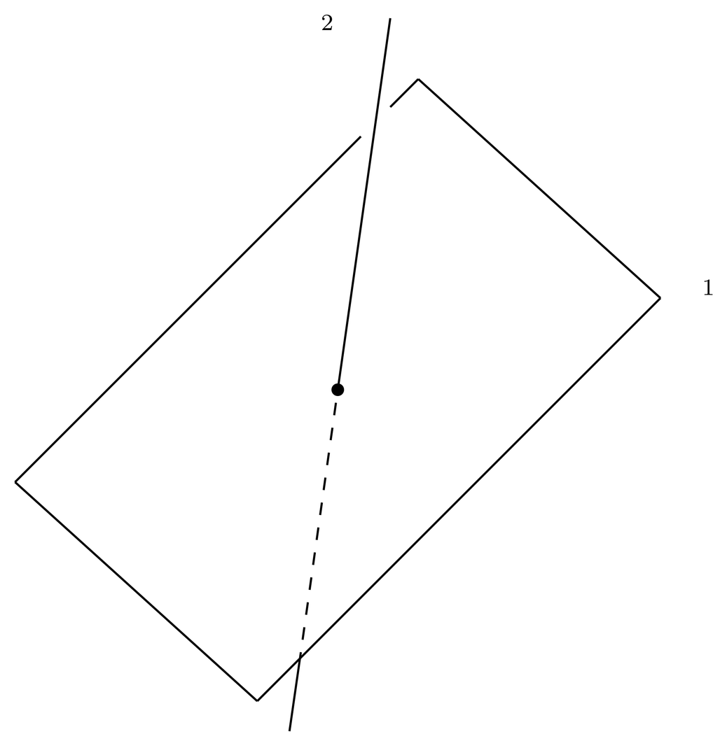
Figure 2:An operator acting on ket space has eigenspaces , associated with its discrete eigenvalues .
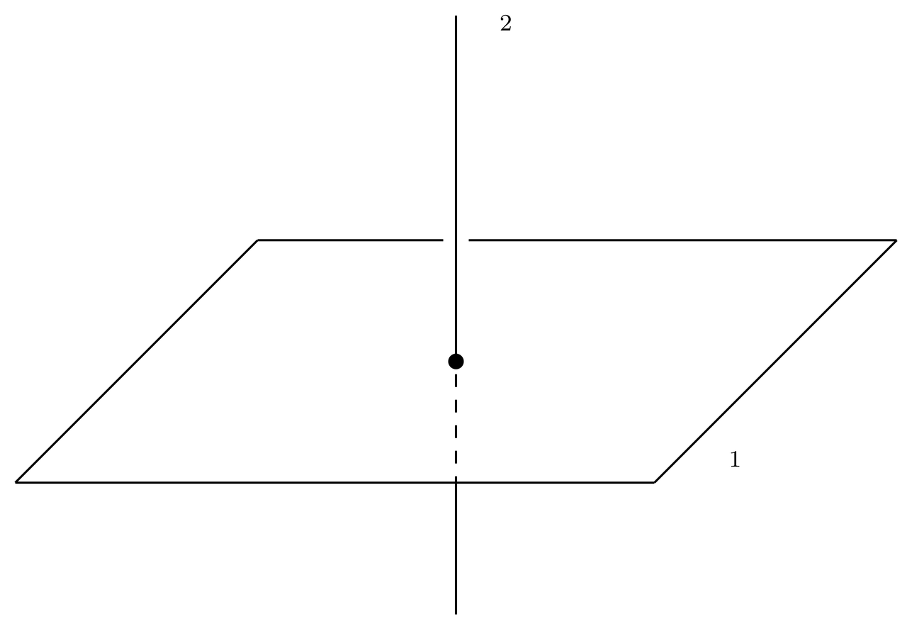
Figure 3:In the case of a Hermitian operator, the eigenspaces are orthogonal.
In the case of the discrete spectrum, the set of kets that satisfy (70) for a given eigenvalue forms a vector subspace of the ket space. This subspace is at least 1-dimensional, but the dimensionality may be higher (even infinite, on infinite-dimensional vector spaces). We will call this subspace the eigenspace of the operator corresponding to the given eigenvalue. If the eigenspace is 1-dimensional, then we say the eigenvalue is nondegenerate, otherwise, that it is degenerate. We refer to the dimensionality of the eigenspace as the order of the degeneracy. This is the same as the number of linearly independent eigenvectors of a given eigenvalue. We can imagine the eigenspaces of the discrete spectrum as illustrated in Figure 2, which shows the eigenspaces for a two-fold degenerate eigenvalue and a nondegenerate eigenvalue (, ).
The Case of Hermitian Operators
In general, there is no simple relation between the eigenkets and eigenbras of an operator, even in finite dimensions. But if an operator is Hermitian, then there are a number of simplifications. We speak for the time being of the discrete spectrum.
First, the eigenvalue is real, so the spectrum in the complex eigenvalue plane is a subset of the real axis. To prove this we take and multiply on the left by , obtaining
Now taking the complex conjugate of this, the left-hand side goes into itself, while the right becomes . Thus we have
Since , this implies .
Second, if , then , so that the eigenbras are the Hermitian conjugates of the eigenkets, and the left and right eigenvalues are equal.
Third, any two eigenkets corresponding to distinct eigenvalues are orthogonal. We state this final property as a theorem:
To prove this, we let and for two eigenkets and and two eigenvalues and . Multiplying the first equation by and the second by , we obtain
Now taking the Hermitian conjugate of the second equation and subtracting from the first, we find
showing that either or else .
In view of this theorem, Figure 3 gives a more accurate picture of the eigenspaces of a Hermitian operator than does Figure 2.
Completeness
In looking at Figs.~Figure 2 and Figure 3 we may imagine that the space in which the eigenspaces lie is three dimensional, so the two eigenspaces (of dimension 2 and 1) “fill up” the whole space. Do the eigenspaces of an operator always “fill up” the space upon which the operator acts? An operator that does this is said to be complete. The answer is no, not even in finite dimensions. For example, the matrix
possesses only one eigenvector, namely,
so it has only a single one-dimensional eigenspace. The matrix (76) is not Hermitian.
On the other hand, in finite dimensions every Hermitian operator is complete. Thus, the sum of the dimensionalities of the eigenspaces is the dimension of the whole space. Since the eigenspaces are orthogonal, by choosing an orthonormal basis in each eigenspace we obtain an orthonormal eigenbasis for the whole space, that is, a set of orthonormal basis vectors that are also eigenvectors of the operator. This is a consequence of the standard methods taught in linear algebra courses for diagonalizing Hermitian matrices, which explicitly produce the orthonormal eigenbasis.
Notice that the orthonormal eigenbasis is not unique. First, if there is any degeneracy (any eigenspace with dimensionality ), then obviously there are an infinite number of ways of choosing an orthonormal basis in that eigenspace. But even in a nondegenerate (one-dimensional) eigenspace, a normalized eigenvector is only determined to within a phase factor.
These nice properties of Hermitian operators are shared by a larger class of normal operators, which will be studied in a homework exercise. Occasionally in quantum mechanics we must deal with the eigenvectors of non-Hermitian operators and worry about their completeness properties. This happens, for example, in the theory of the Dirac equation.
The Direct Sum; Orthonormal Eigenbases
Suppose we have some vector space , and suppose and are vector subspaces of that have no element in common except 0, such as the spaces we see in Figs.~Figure 2 and Figure 3. Then we say that the direct sum of and , denoted , is the set of vectors that can be formed by taking linear combinations of vectors in the two subspaces. That is,
The direct sum is itself a vector subspace of . One can also think of the direct sum as the span of the set of vectors formed when we throw together a basis in with a basis in . Thus, we have
This is not the most abstract definition of the direct sum, but it is the one we will use.
We can now express the completeness property in finite dimensions in terms of the direct sum. Let be an operator acting on a finite-dimensional space . Let the eigenvalues of be , and let be the -th eigenspace, that is,
Then is complete if
In finite dimensions, any Hermitian is complete, and moreover it decomposes the original Hilbert space into a collection of orthogonal subspaces, the eigenspaces of the operator.
Let us choose an orthonormal basis, say , in each of the subspaces , where is an index labeling the orthonormal vectors in the subspace, so that . This can always be done, in many ways. Then, since the various subspaces are themselves orthogonal, the collection of vectors for all and forms an orthonormal basis on the entire space , so that
These kets are eigenkets of ,
that is, they constitute an orthonormal eigenbasis. Furthermore, we have the resolution of the identity,
corresponding to the chosen orthonormal eigenbasis of the complete Hermitian operator . Also, the operator itself can be written in terms of this eigenbasis,
This follows if we let both sides of this equation act on a basis vector , whereupon the answers are the same. By linear superposition, the same applies to any vector. Thus, both sides are the same operator.
Spectral Properties in Infinite Dimensions
Here we make some remarks about infinite-dimensional ket spaces and illustrate the kinds of new phenomena that can arise.
In infinite dimensions, there exist Hermitian operators that are not complete. To cover this case, we define a complete Hermitian operator as an observable. This terminology is related to the physical interpretation of observables in quantum mechanics, as explained in 02. The Postulates of Quantum Mechanics. In practice we seldom deal with incomplete Hermitian operators in quantum mechanics.
We now use examples from one-dimensional wave mechanics to illustrate some phenomena that can occur in infinite dimensions. The Hilbert space of wave functions in one dimension consists of normalizable functions with the scalar product,
We will present four examples of operators and their spectral properties.
The first is the one-dimensional harmonic oscillator with Hamiltonian,
which is a Hermitian operator. The energy eigenvalues are
so that the spectrum consists of a discrete set of isolated points on the positive energy axis, as illustrated in Figure 1(a). The eigenfunctions are normalizable (they belong to Hilbert space) and orthogonal for different values of the energy. Thus they can be normalized so that
These eigenfunctions are nondegenerate and complete, so we have a resolution of the identity,
Not all Hermitian operators on an infinite dimensional space have a discrete spectrum. As a second example, consider the momentum operator in one dimension, which is . (We put a hat on the operator, to distinguish it from the eigenvalue .) The momentum is a Hermitian operator (see below). The eigenvalue-eigenfunction equation for this operator is
where is the eigenfunction with eigenvalue . This equation has a solution for all values, real and complex, of the parameter ,
where is a constant. If has a nonzero imaginary part, then diverges exponentially as or , so the “eigenfunction” is rather badly behaved. It is certainly not normalizable in this case. But even if is purely real, the function is still not normalizable, so it does not represent a physically allowable state (a vector of Hilbert space). The momentum operator does not have any eigenvectors that belong to Hilbert space, much less a basis.
One way to handle this case, which provides a kind of generalization of the nice situation we find in finite dimensions, is to regard every real number as an eigenvalue of , which means that the spectrum of is the entire real axis (in the complex -plane). See Figure 1(b) for an illustration of the spectrum of the free particle Hamiltonian, which is the portion of the real axis. Recall that in finite dimensions a Hermitian operator has only real eigenvalues. This is an example of the continuous spectrum. Also, the eigenfunctions that result in this case are orthonormal and complete in a certain sense, but as noted they do not belong to Hilbert space. We obtain an orthonormal basis, but it consists of vectors that lie outside Hilbert space.
We adopt a normalization of the eigenfunctions (that is, we choose the constant in (92) so that
because this implies a convenient normalization relation,
where we write the function in ket language as (giving only the eigenvalue). The eigenfunctions of the continuous spectrum are orthonormal only in the -function sense. They are also complete, in the sense that an arbitrary wave function can be expanded as a linear combination of them, but since they are indexed by a continuous variable, the linear combination is an integral, not a sum. That is, given , we can find expansion coefficients such that
We know this because (95) is essentially a Fourier transform, whose inverse is given by
We see that the “momentum space wave function” is otherwise the scalar product .
Another example of an operator with a continuous spectrum is the position operator (again using hats to denote an operator). This operator acting on wave functions means, multiply by . If we denote the eigenfunction of this operator with eigenvalue by , then the eigenvalue equation is
or,
This implies either or , so is a “function” that is zero everywhere except possibly at . We interpret this situation in terms of the Dirac delta function, by writing the solution as
Again, the spectrum is continuous and occupies the entire real axis; again, the “eigenfunctions” are of infinite norm and obey the continuum orthonormality condition,
where we write the function in ket language as (giving only the eigenvalue). In addition, we have the identity,
We see that the wave function is otherwise the scalar product . Substituting this back into (101) and using (100), we have
or, since is arbitrary,
Finally, since is arbitrary, we can strip it off, leaving
the resolution of the identity in the case of the continuous eigenbasis of the position operator.
We can also get the resolution of the identity in the momentum basis. Since for any , we have . Substituting these and (96) into (95), we have
or, stripping off both on the left and on the right,
Equations (104) and (106) illustrate resolutions of the identity in the case of the continuous spectrum.
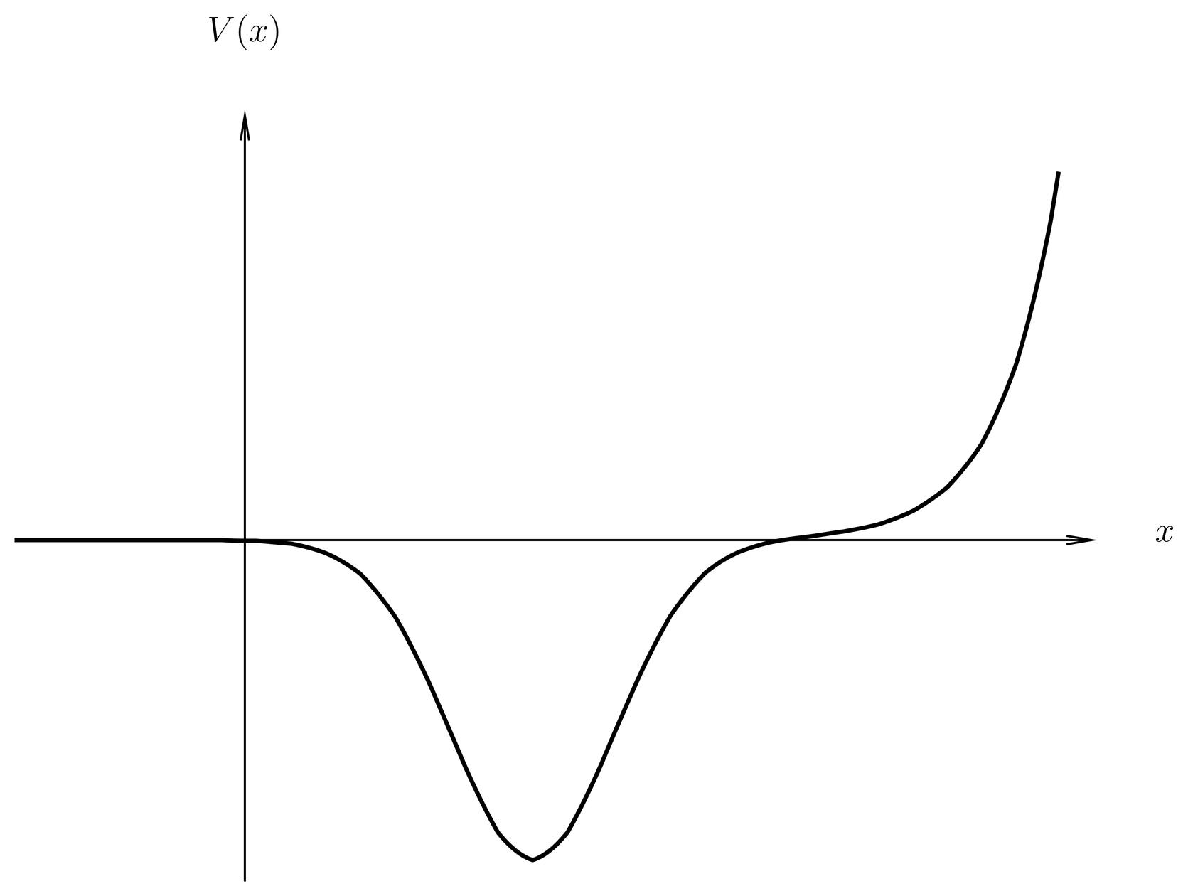
Figure 4:A potential in 1-dimension with both bound and unbound eigenstates.
For a final example, let us consider the 1-dimensional potential illustrated in Figure 4, which has a well followed on the right by an infinitely high barrier. The purpose of the barrier is simply to make the unbound energy eigenfunctions nondegenerate, which simplifies the following discussion. In a potential such as this, we expect there to be some number of bound eigenfunctions in the potential well, which have negative energies . These eigenfunctions are normalizable, because the wave functions die off exponentially outside the well, and we can normalize them according to , as with the discrete spectra discussed above. But there will also be unbound eigenfunctions corresponding to any energy ; these eigenfunctions become free particle wave functions at large negative , and therefore have infinite norm. We normalize them according to . Finally, all bound states are orthogonal to all continuum states, . Thus, the completeness relation in this case has the form,
In this case we have an example of a mixed spectrum, with some discrete and some continuous eigenvalues. The spectrum consists of a discrete set of points on the negative energy axis, plus the entire positive energy axis .
More complicated kinds of spectra also occur. It is possible to have discrete states imbedded in the continuum, not in real physical problems but in approximations to them, in which certain interactions are switched off. When all the physics is taken into account, such discrete states typically move off the real axis, and become resonances with a finite lifetime. Examples of this occurs in the autoionizing states of helium, or in the radiative decay of excited atomic states. See 44. Natural Line Width, Long-Time Behavior and the Lamb Shift. It is also possible to have a discrete spectrum in which the eigenvalues are not isolated, as in the random potentials that occur in the theory of Anderson localization, an important topic in solid state physics.
Generalizations about Spectra, Eigenspaces and Eigenbases
On a finite-dimensional Hilbert space, all Hermitian operators have a discrete spectrum (and they are moreover complete). The continuous and more complicated types of spectra arise only in the infinite dimensional case.
In the infinite dimensional case, each eigenvalue of the discrete spectrum corresponds to a definite eigenspace, a subspace of the Hilbert space consisting of normalizable eigenvectors of the Hermitian operator in question. If such an eigenspace is finite dimensional, then it possesses a finite, discrete basis of normalizable eigenvectors, as does any finite-dimensional Hilbert space. If an eigenspace of the discrete spectrum is infinite dimensional, then it is an infinite dimensional subspace of a Hilbert space and is therefore an infinite dimensional Hilbert space in its own right. This means that it is possible to choose a discrete basis of normalizable vectors that span this space, but that it may be convenient in practice to choose other types of bases, such as a continuous basis, consisting of unnormalizable vectors outside Hilbert space, or a mixed basis, or other possibilities.
An example of an infinite dimensional eigenspace of an operator with a discrete spectrum is given by the parity operator acting on wave functions in one dimension. The two eigenspaces consist of wave functions that are even and odd under , corresponding to the eigenvalues +1 and -1 of the parity operator, and both are infinite dimensional.
In the continuous spectrum, there is no subspace of the Hilbert space corresponding to a given eigenvalue. For example, in the case of the free particle in one dimension with Hamiltonian , for a given there are two linearly independent eigenfunctions, and , where . But these eigenfunctions are not normalizable, and do not belong to Hilbert space. Since there is no linear combination of these eigenfunctions that is normalizable, they do not specify a subspace of Hilbert space. On the other hand, any interval in the continuous spectrum does correspond to a subspace of the Hilbert space. This subspace consists of normalizable vectors that can be represented as linear combinations of the unnormalizable eigenvectors whose eigenvalues lie in the given interval.
For example, let be an interval of the momentum axis. Then normalizable wave functions whose Fourier transform vanishes outside the interval form a subspace of the Hilbert space of normalizable wave functions .
Concepts like this are familiar in electronics. A circuit that passes a signal in a certain frequency range while rejecting frequency components outside that range is analogous to a projection operator in quantum mechanics that projects onto a certain interval of the momentum axis . The main difference is that one works in the time domain and the other in the spatial domain [when acting on wave functions ].
The concept of a subspace corresponding to an interval of the continuous spectrum plays a role in the measurement postulates of quantum mechanics, as we will see in 02. The Postulates of Quantum Mechanics.
Proving of Hermiticity of the Momentum
To show that the momentum operator is Hermitian on the Hilbert space of wave functions with scalar product (86), we appeal to the definition of Hermiticity in the form (63). Letting and be two wave functions, we have
by integration by parts. The first integral vanishes if and go to zero as , something we normally expect for normalizable wave functions (but see Mathematical Notes). The final integral is
which completes the proof. A similar proof can be given for Hamiltonians of the form . More simply, once we know that and are Hermitian, we can use the general rules presented in these notes (for example, (60) and A Function of an Observable)) to conclude that the sum of any real function of and any real function of is Hermitian.
Orthonormality and Completeness in the General (Degenerate) Case
We return now to the general case of a complete Hermitian operator (an observable) acting on an infinite-dimensional Hilbert space. In general, the spectrum consists of a discrete part, with eigenvalues , and a continuous part, with eigenvalues that are functions of some continuous variable . (We could choose , but sometimes it is convenient to use another continuous parameter upon which the eigenvalue depends. For example, we may wish to use the momentum instead of the energy to parameterize continuum energy eigenvalues and eigenfunctions.) In addition, we must in general introduce another index to resolve degeneracies in degenerate subspaces; for simplicity we will assume that is a discrete index, although in some problems this would be continuous, too. Then the orthonormality conditions have the form,
and the completeness relation has the form,
As a specific example of these relations, consider the hydrogen atom in the electrostatic model, in which we neglect the electron spin. The bound state wave functions are in the usual notation, which we write in ket language as . We normalize these so that . In addition, there are unbound (and unnormalizable) eigenfunctions of energy , which we write in ket language as . We normalize these so that . Also, the bound states are orthogonal to the unbound states, . Then the completeness relation has the form,
The generalized orthonormality and completeness relations we have just presented are examples of an important theorem, which we now quote:
This eigenbasis must include states of infinite norm, if the observable possesses a continuous spectrum.
Simultaneous Eigenbases of Commuting Observables
Next we turn to an important theorem, applications of which will occur many times in this course:
For simplicity we will work on a finite-dimensional Hilbert space . We begin with the case of two observables. In the first part of the proof, we assume we have two Hermitian operators , that commute. We wish to prove that they possess a simultaneous eigenbasis.
Consider the -th eigenspace of the operator , and let be a eigenket in this eigenspace, so that
Then by multiplying by and using the fact that , we easily conclude that
in which we use parentheses to emphasize the fact that the ket is also an eigenket of with the same eigenvalue, . Note the possibility that could vanish, which does not, however, change any of the following argument. We see that if any ket belongs to the subspace , then so does the ket .
To complete the proof we need the concept of the restriction of an operator to a subspace. In general, it is only meaningful to talk about the restriction of an operator to some subspace of a larger space upon which the operator acts if it should happen that the operator maps any vector of the given subspace into another vector of the same subspace. In this case, we say that the subspace is invariant under the action of the operator.
In the present example, both operators and leave the subspace invariant. As for , this follows from (115), which is in effect the definition of . As for , this follows from (116). Let us denote the restriction of and to the subspace by and , respectively. Then, according to (115), is a multiple of the identity, , where stands for the identity operator acting on the subspace. The operator cannot be expressed so simply, but it is a Hermitian operator, since was Hermitian on the larger space . Since we are assuming that is finite-dimensional, so is , and therefore is complete on . Therefore possesses an orthonormal eigenbasis in , say,
where . Here is considered fixed, and if there are any degeneracies of , they are indicated by repetitions of the eigenvalues for different values of .
If we now construct the bases in a similar manner for each value of , then we obtain a simultaneous, orthonormal eigenbasis for both and on the whole space . Notice that there may be degeneracies of that cross the eigenspaces of , that is, there may be repetitions in the values for different values of .
To prove the converse of Theorem~Theorem, we assume that and possess a simultaneous eigenbasis. We sequence the kets of this eigenbasis according to some index , and write
In these formulas, we do not assume that the eigenvalues or are distinct for different values of ; degeneracies are indicated by repetitions of the values or for different values of . Now from (118) it follows immediately that
or,
But since the kets form a basis, (120) implies . QED. (The extension of Theorem~Theorem will be left as an exercise.)
An important corollary of Theorem~Theorem occurs when some eigenvalue of is nondegenerate, so that is 1-dimensional. In that case, all kets in are proportional to any nonzero ket in . Thus, if we let be some standard, normalized eigenket of with eigenvalue , then (116) tells us that must be proportional to , say,
for some number . We see that is an eigenvalue of , and is an eigenket, although the theorem does not tell us the value of . The number must be real, since is Hermitian. We summarize these facts by another theorem.
The proof of the extension will be left as an exercise.
As an example of this theorem, consider a Hamiltonian that commutes with parity, . According to the theorem, every nondegenerate eigenstate of the Hamiltonian is necessarily a state of definite parity (even or odd), that is, it is an eigenstate of parity. Recall that in the one-dimensional harmonic oscillator, the energy eigenstate for are even under parity, while those for are odd.
Projection Operators
We turn now to the subject of projection operators. We say that an operator is a projection operator or a projector if it is an observable that satisfies
(On account of this equation, we say that is idempotent, from Latin idem = same,' and *potens* = powerful.') It follows immediately from this definition that the eigenvalues of are either 0 or 1, for if we write
then by (122) we have
or,
Thus, either or ; we exclude the latter possibility, since eigenkets are supposed to be nonzero, and therefore conclude that either or . Therefore breaks the Hilbert space into two orthogonal subspaces,
such that annihilates any vector in , and leaves any vector in invariant. We say that is the space upon which projects.
Projection operators arise naturally in the eigenvalue problem for an observable . For simplicity, assume that has a discrete spectrum, so that we can write
where is an orthonormal eigenbasis of , with an arbitrarily chosen orthonormal basis in each eigenspace . We then define
It is left as an exercise to show that the operator actually is a projector, and that it projects onto eigenspace of . The set of projectors for different also satisfy
As we say, the projectors form an orthogonal set.
It follows immediately from the definition (128) and the resolution of the identity (84) that
which is yet another way of writing the completeness relation for .
One can also express the operator itself in terms of its projectors. We simply let act on both sides of the resolution of the identity, (84), and use (127) and (128). The result is
In the case of the continuous spectrum, a projector can be associated with an interval of the parameter describing the continuous spectrum. For if we normalize the eigenkets of some operator as in (112), then it is easy to show that the operator
is a projector, and that the projectors for two intervals and are orthogonal if and only if and do not intersect.
The use of projection operators is generally preferable to the use of eigenvectors, because the latter are not unique. Even when nondegenerate and normalized, an eigenvector is subject to multiplication by an arbitrary phase factor, and in the case of degeneracies, an orthonormal basis can be chosen in the degenerate eigenspace in many ways. However, it is easy to show that the projector defined in (128) is invariant under all such redefinitions, as should be obvious from the geometrical fact that projects onto . Also, in the continuous spectrum there are no eigenvectors that belong to Hilbert space (which means that they are normalizable and hence physical), but the projection operators (132) are always defined and well behaved.
A Function of an Observable
The concept of a function of an observable arises in many places. We begin with the case of the discrete spectrum. If is an observable with discrete eigenvalues and corresponding projectors , we define by
It is easy to show that when is a polynomial or power series, is the same as the obvious polynomial or power series in the operator ; but (133) defines a function of an observable in more general cases, such as the important cases , or even . When has a continuous spectrum, we can no longer express in terms of projectors, but we can write it in terms of the complete basis of eigenkets, in the notation of (113). In this case we have
Number Terminology
In quantum mechanics we often have to draw the distinction between an operator and its eigenvalues, or an operator (a quantum observable) and its classical counterpart, which is number. Some terminology due to Dirac is useful for such purposes. Dirac refers to an ordinary (real or complex) number as a “-number,” while he calls an operator a “-number.” We will often use this terminology.
Operators and Kets versus Matrices and Vectors
We now consider the relation between abstract kets, bras, and operators and the vectors and matrices of numbers that are used to represent those abstract objects. Consider, for example, the eigenvalue problem for a Hermitian operator . To convert this into numerical form, we simply choose an arbitrary orthonormal basis , , and insert a resolution of the identity before the ket on both sides. We then multiply from the left with bra , to obtain
Thus, with
we have
The matrix elements form a Hermitian matrix,
and the eigenvalue problem becomes that of determining the eigenvalues and eigenvectors of a Hermitian matrix. Now the eigenvector , as a column vector of numbers, contains the components of the eigenket with respect to the chosen basis. Of course, if the Hilbert space is infinite-dimensional, then the matrix is also infinite-dimensional. In practice, one usually truncates the infinite-dimensional matrix at some finite size, in order to carry out numerical calculations. One can hope that if the answers seem to converge as the size of the truncation is increased, then one will obtain good approximations to the true answers (this is the usual procedure).
The above is for a discrete basis. Sometimes we are also interested in a continuous basis, for example, the eigenbasis of the operator . Again working with the eigenvalue problem , we can insert a resolution of the identity before on both sides, and multiply from the left by . Then using the orthogonality relation (100), we obtain
or,
where
We see that the “matrix element” of an operator with respect to a continuous basis is nothing but the kernel of the integral transform that represents the action of that operator in the given basis. (The kernel of an integral transform such as (140) is the function that appears under the integral.)
Traces
The trace of a matrix is defined as the sum of the diagonal elements of the matrix. Likewise, we define the trace of an operator acting on a Hilbert space as the sum of the diagonal matrix elements of with respect to any orthonormal basis. Thus, in a discrete basis we have
One can easily show that it does not matter which basis is chosen; the trace is a property of the operator alone. One can also use a continuous basis to compute the trace (replacing sums by integrals). The operator in (142) need not be Hermitian, but if it is, then the trace is equal to the sum of the eigenvalues, each weighted by the order of the degeneracy,
where is the order of the degeneracy of . This is easily proven by choosing the basis in (142) to be the orthonormal eigenbasis of . But if has a continuous range of eigenvalues, then the result diverges (or is not defined). Even if the spectrum of is discrete, the sum (143) need not converge.
The trace of a product of operators is invariant under a cyclic permutation of the product. For example, in the case of three operators, we have
This property is easily proven. Another simple identity is
If and are operators, we are often interested in a kind of “scalar product” of with , especially when we are expressing some operators as linear combinations of other operators (the Pauli matrices, for example). The most useful definition of a scalar product of two operators is
where the final expression involves the matrix elements of and with respect to an arbitrary orthonormal basis. Thus, the scalar product of an operator with itself is the sum of the absolute squares of the matrix elements,
which vanishes if and only if .
Mathematical Notes
We collect here some remarks of a mathematical nature on the preceding discussion. For a precise treatment of the mathematics involved, see the references.
The set of normalizable wave functions is infinite-dimensional because given any finite sequence of normalizable wave functions, , one can always find a new normalizable wave function that is linearly independent of those given.
A Hilbert space is a complex, normed vector space that is complete. The latter property means that all Cauchy sequences converge to a point of the space. This property is automatic in finite dimensions. In addition, many authors require a Hilbert space to be separable, which means that it possesses a countable basis. Sakurai (in Modern Quantum Mechanics) is mistaken when he says that a Hilbert space has an uncountable basis; he is thinking of the “bases” of the continuous spectrum, such as the set , but these basis wave functions are not normalizable and do not belong to Hilbert space. In field theory, one must deal with spaces that are not separable (since they possess uncountable bases of normalizable vectors, but not countable ones). Such spaces are called Fock spaces.
Properly speaking, functions do not stand in one-to-one correspondence with elements of Hilbert space. The functions must be measurable, and two functions that differ by a subset of measure zero are considered equivalent. Thus, it is really an equivalence class of wave functions that corresponds to a state vector . All these wave functions, however, give the same results in their physical predictions (such as the probability of finding a particle on some interval). This is related to the fact that one cannot measure a wave function at a point, so there is no physical way to detect the difference between two wave functions that differ on a subset of measure zero.
Sometimes Hermitian operators are also called self-adjoint; to be precise about this terminology, on a finite-dimensional Hilbert space “Hermitian” and “self-adjoint” are equivalent, but on an infinite-dimensional space this is true only if certain assumptions are made about the properties of the operators and their domains of definition.
The usual Hermitian operators encountered in quantum mechanics (for example, Hamiltonians) are complete, although the mathematical proof is often technical. In fact, the completeness property is intimately tied up with the physical interpretation of the measurement process, since (according to the usual interpretation of measurement) if a measurement were to correspond to an incomplete operator, it would mean that measuring all possible outcomes would result in a total probability less than unity. In this course (and in most of the literature on quantum mechanics) we assume the completeness of all Hermitian operators we encounter without further comment.
Regarding the first integral on the right in (108), which must vanish in order to show that , we note that normalizability does not imply that a wave function approaches zero as . At issue here is the fact that the momentum operator is unbounded, that is, it maps some normalizable wave functions into unnormalizable ones (taking them out of Hilbert space). If, however, both and are normalizable, then the integral in question does vanish.
References
The standard early reference for physicists on the formalism of quantum mechanics is P. A. M. Dirac, The Principles of Quantum Mechanics, 4th ed (Oxford University Press, Oxford, 1974), while for mathematicians it is John von Neumann, Mathematical Foundations of Quantum Mechanics (Princeton University Press, Princeton, 1955) (this is the English translation of the German original). Modern textbooks that devote more than the usual attention to mathematical questions include Albert Messiah, Quantum Mechanics vols. I and II (John Wiley, New York, 1966) (translation of French original), and Leslie E. Ballentine, Quantum Mechanics: A Modern Development (World Scientific, Singapore, 1998). The standard modern reference on the mathematics of quantum mechanics is Michael Reed and Barry Simon, Functional Analysis revised ed (Academic Press, New York, 1980), and, by the same authors, Fourier Analysis, Self-Adjointness (Academic Press, New York, 1975). See also Quantum Mechanics in Hilbert Space by Eduard Prugove\v cki (Dover, Mineola, New York, 1981).
Problems
Problem 1.
Consider the matrices:
Matrices , and are called the Pauli matrices. We will also denote them , , .
(a) Show that
where is understood to be multiplied by , where we use the summation convention (see The Summation Convention), and where is the completely antisymmetric Levi-Civita symbol (see The Levi-Civita Symbol in Three Dimensions, and ask if you don’t understand, since this notation will be used frequently in the course). Notice that (149) implies
and
where the curly brackets are the anticommutator.
What we mean by a vector operator is a vector of operators, for example, , where , and are operators. Now given any two vector operators , that commute with but not necessarily with each other, use (149) to show that
where
We think of as a “vector” of matrices.
Two vector operators are considered to commute if all of their components commute. Note that in general, , and .
(b) Let be an arbitrary unit vector and an arbitrary angle. Show that
In this course we will often drop the , it being understood that a scalar like is multiplied by the identity matrix.
Problem 2.
Lie algebraic techniques for operators.
(a) Consider two operators , that do not necessarily commute. Show that
Hint: Replace by , where is a parameter, and let the left-hand side be . Find a differential equation satisfied by , and solve it. Alternatively, expand in a Taylor series in .
(b) Let be an operator that depends on time. Derive the following operator identity:
where
where is an arbitrary operator. Also, . Do not assume that commutes with . We will use this identity when we study the nonrelativistic limit of the Dirac equation.
Problem 3.
Pauli matrices and traces.
(a) If and are square matrices, show that
Also prove (144).
(b) Show that . It may be easiest just to use the definitions (148). Then use (149) to find a simple expression for .
(c) The set of four matrices, form a basis in the space of matrices, that is, an arbitrary matrix can be expressed as a linear combination of these four matrices. Thus, if is an arbitrary matrix, it can be expressed as
This follows from the fact that and the three are linearly independent, as can be seen just by looking at the four matrices. Find neat expressions for the expansion coefficients, and . Do this by taking traces, or by multiplying by a Pauli matrix and then taking traces. Also show that is Hermitian if and only if , are real.
(d) Now suppose that is nonzero in only the slot, where it has a 1. That is, let
Use this in (159) to find a nice expression for (summation convention everywhere, so sum on in this expression) in terms of Kronecker deltas.
Problem 4.
Some easy proofs from the notes.
(a) Show that (50) follows from (49).
(b) Prove (57), (60), and (61).
(c) Prove that the product of two Hermitian operators is Hermitian if and only if they commute.
(d) Show that
Problem 5.
The problem of finding the eigenkets and eigenbras of an arbitrary operator is more complicated and full of exceptions than in the case of Hermitian operators. There are, however, other classes of operators that share many of the nice properties of Hermitian operators. These include anti-Hermitian and unitary operators.
We define an operator to be normal if it commutes with its Hermitian conjugate, . Notice that Hermitian, anti-Hermitian, and unitary operators are normal. In the following you may assume that you are working on a finite-dimensional Hilbert space.
(a) Show that if is normal, and for some nonzero , then . Thus, the eigenbras of are the Hermitian conjugates of the eigenkets, and the left spectrum is identical to the right spectrum. Hint: it is not necessary to introduce orthonormal bases or anything of the kind.
(b) Show that the eigenspaces corresponding to distinct eigenvalues of a normal operator are orthogonal. This is a generalization of the easy and familiar proof for Hermitian operators.
Problem 6.
Some things that will be needed in subsequent problems. In parts (a)--(c) of this problem you may assume that you are working on a finite-dimensional Hilbert space.
(a) If is an observable, show that
where is the projector onto the -th eigenspace of . This shows that the projector is a function of the operator (see A Function of an Observable).
(b) Show that if
for all , then . ( is not necessarily Hermitian.) Would this be true on a real vector space? (A real vector space is one in which the coefficients allowed in forming linear combinations of basis vectors are real. In a complex vector space, such as Hilbert space, these coefficients are allowed to be complex.)
Problem (c).
Let be a linear operator, and let . Show that for all kets if and only if is unitary.
Problem (d).
Consider now the Hilbert space for a particle moving in one dimension, which is infinite-dimensional. Let be the usual harmonic oscillator eigenbasis, with . Define an operator by
Show that if , then . Then show that
Thus has a left inverse, and it is . Does have a right inverse? Is unitary?
This problem shows that in an infinite dimensional Hilbert space, if an operator preserves the norm of all vectors, and if it possesses an inverse (both left and right), then it is unitary.
Problem 7.
Let be a real vector space with a positive definite scalar product. If and are vectors in , we denote their scalar product by . This is like the scalar product in the Hilbert spaces of quantum mechanics, except only real coefficients are allowed when forming linear combinations of vectors. We interpret as the square of the length of the vector . Show that the Schwarz inequality (\eqr\cn.28) implies that the shortest distance between two points is a straight line.