17. Hydrogen and Hydrogen-Like Atoms
Introduction
There is an amazing amount of physics in the hydrogen atom. The simplest model, the electrostatic model that we consider in these notes, is an exactly solvable problem that reveals the gross structure of the hydrogen atom and explains the formulas of Balmer and Rydberg for its spectral lines. Later, in 25. Fine Structure in Hydrogen and Alkali Atoms, we will consider corrections due to relativity and spin, which produce the fine structure in the spectrum of hydrogen as well as giving us an introductory view of relativistic quantum mechanics. Then, in 27. Hyperfine Structure in Atoms, we will consider the magnetic interactions between the atomic electron and the magnetic dipole moment of the nucleus, which are otherwise known as hyperfine effects. These are important for many applications ranging from atomic clocks to astrophysics. Later we study the Lamb shift, a shift in the atomic energy levels due to the interaction of the atomic electron with the quantized electromagnetic field, which is most notable in the case of hydrogen where it splits the degeneracy of the and states. Finally, in 50. Solutions of the Dirac Equation and Their Properties{} we consider the exact solution of the hydrogen atom for the Dirac equation, the relativistic wave equation for the electron, as well as (in 49. The Foldy-Wouthuysen Transformation) the expansion of solutions of the Dirac equation in powers of , recovering thereby all the fine structure effects examined earlier in 25. Fine Structure in Hydrogen and Alkali Atoms. Hydrogen is also a basic model for the physics of atoms, providing a context and a reference for all of atomic physics and as well as for the physics of collections of atoms, including molecules and most systems of interest in condensed matter physics.
In addition to hydrogen itself in these notes we will also consider hydrogen-like atoms, that is, atoms with a nucleus of some charge and a single electron. This includes the ion , singly ionized helium, also called hydrogen-like helium; the ion , doubly ionized lithium, also called hydrogen-like lithium, etc. As usual in atomic physics, we denote the nuclear charge by , which ranges from 1 for hydrogen to 92 for uranium and beyond.
Hydrogen in the History of Quantum Mechanics
Hydrogen played a central role in the history of quantum mechanics. By the 1880’s Balmer and Rydberg had found an empirical formula fitting the observed spectral lines in hydrogen,
where is the wavelength of the radiation emitted, is a constant that can be determined from the spectroscopic data, and and are positive integers such that . In 1913 Bohr showed that the Rydberg formula (1) could be explained by demanding that the orbits of the electron in hydrogen are quantized, that is, restricted to those for which the classical action is an integer multiple of , and that when atoms jump from one quantized orbit to another, the frequency of the photon emitted is given by Einstein’s formula . This was not obvious, because this frequency is not the same as the orbital frequency of either the old or new orbit. Bohr’s theory showed that the Rydberg constant in (1) was given by
a result that agreed well with the spectroscopic data. The value of was known by that time due to the work of Planck and others on black body radiation. Bohr’s theory explained other things as well, such as the dependence of the Rydberg constant on the nuclear charge in single-electron atoms [the formula (2) applies only to hydrogen].
In 1916 Sommerfeld used a relativistic generalization of Bohr’s method of quantizing orbits to explain (apparently) the fine structure of hydrogen, although we now know that this calculation gave the correct answer somewhat by accident. Sommerfeld did not know about spin and the version of the old quantum theory he was using had some inadequacies, but by a kind of a miracle the answers turned out to agree with experiment. In spite of these misconceptions, however, Sommerfeld was correct in realizing that the fine structure was a relativistic correction to the dynamics of hydrogen.
When the first version of genuine quantum mechanics appeared 1925, in the form of Heisenberg’s matrix mechanics, one of the first problems solved was the hydrogen atom. It is entirely nontrivial to do this within the framework of matrix mechanics, but the solution was given in 1926 in a brilliant paper by Pauli. Pauli had been primed for the task by his earlier work on the hydrogen molecule-ion () in the old quantum theory. Soon afterward the Schr"odinger equation and wave mechanics appeared, and Schr"odinger himself solved his equation for the hydrogen atom, much along the same lines as presented in these notes.
By this time the concept of spin had been introduced and comprehended much in its modern form, by Kronig, Pauli and others, and it was understood that spin was a part of some as yet incomplete understanding of relativistic quantum mechanics. A major breakthrough was made by Dirac in 1927, with his relativistic wave equation for the electron. Dirac did not solve his equation for the hydrogen atom, instead that was done by Darwin in 1928. This exact solution of the Dirac equation reproduced all of the fine structure effects in hydrogen to within the experimental accuracy available at that time. (When asked once why he did not solve his own equation for hydrogen, Dirac replied that he was afraid to, for fear that the answers would come out wrong and ruin his theory.)
The Dirac equation predicts an exact degeneracy between the and levels of hydrogen, but spectroscopists in the 1930’s began to suspect that there might be a splitting between them, one that was just beyond the resolution available with optical techniques. At the same time several theorists began to suspect that this splitting was due to the interaction of the atomic electron with the quantized electromagnetic field, one in which the atomic electron first emits and then reabsorbs a photon. The problem was that quantum electrodynamics of that day inevitably led to infinities in all higher order perturbation calculations, including this one, so that it was impossible to get a theoretical number without overcoming the difficulty of the infinities. But after World War II experimentalists pushed the story forward with dramatic new results. In 1947, using newly developed microwave techniques, Lamb and Retherford not only verified that there is indeed a splitting between these levels, but they also measured it to high accuracy. On hearing about this, Hans Bethe carried out a calculation of the Lamb shift, finding good agreement with experiment. Bethe’s calculation was nonrelativistic and somewhat heuristic, but his calculation did show that it was possible to make sense of the difference between infinite quantities to obtain finite answers that agree with experiment. Then the challenge was on to do the same calculation correctly, with fully relativistic quantum mechanics and the new ideas of renormalization. This was carried out by French and Weisskopf, Feynman, and others, providing one of the earliest and most dramatic successes of renormalization theory.
Atomic Units
Atomic units are units in which , where is the electron mass and is the charge of the proton, as usual in this course. They are particularly convenient in atomic problems as a way of getting rid of the clutter of constants that would appear in other units, and for helping us visualize the order of magnitude of various expressions. For example, the atomic unit of distance is the Bohr radius, the size of the hydrogen atom. Similarly, the atomic unit of velocity is the velocity of the electron in the ground state of hydrogen, the unit of energy is twice the ionization potential of hydrogen, the unit of frequency is the frequency of the electron’s orbit in the ground state of hydrogen, etc. There is a unique unit of distance, energy, time, momentum, etc., that can be constructed out of , and , so that all of these become just 1 in atomic units. These quantities were given in Table 1, an expanded version of which we present here in Table 1.
Table 1:Atomic units of distance, energy, time, etc.
Dimension | Unit | Value |
|---|---|---|
distance | ||
energy | ||
velocity | ||
momentum | ||
angular momentum | ||
frequency | ||
time |
Notice that the energy of the ground state of hydrogen is in atomic units while the period of the electron orbit in the ground state is (that is, in ordinary units). Notice also that the speed of light in atomic units is
The Electrostatic Model
In these notes we shall use the electrostatic model for hydrogen-like atoms, in which the electron and nucleus interact by an electrostatic force, which is determined by the instantaneous positions of the particles. The electrostatic model is an approximation to electrodynamics in which one neglects the retardation in the communication between the particles, magnetic effects, and the effects of radiation. As a part of the electrostatic model we shall also assume the electron motion is nonrelativistic, something that is justified in the case of hydrogen, for which the velocity of the electron in the ground state is , as shown by Table 1. We have no choice in this matter, since we have only studied the nonrelativistic Schr"odinger equation so far, and we do not know how to treat fully relativistic quantum problems. Under these assumptions, we have a two-body problem as described in Two-Body Central Force Motion, in which the potential is
Thus, version~2 [see (11)] of the radial Schr"odinger equation is
where is the reduced mass of the electron-nucleus system. In the case of ordinary hydrogen with a proton as the nucleus, the reduced mass differs from the true electron mass by less than one part in 103, and for heavier atoms the fraction is even smaller. We shall retain the distinction between and , but numerically they are very close.
Solving the Radial Schr"odinger Equation
To put this equation into dimensionless form we shall adopt what we call modified atomic units, which are obtained from atomic units by making the replacements and . Modified atomic units are units in which . The change has only a small effect, but gives all the units a dependence on , which is worth noting. Modified atomic units are summarized in Table 2.
Table 2:Modified tomic units of distance, energy, time, etc., useful for treating hydrogen-like atoms.
Dimension | Unit | Value |
|---|---|---|
distance | ||
energy | ||
velocity | ||
frequency | ||
time |
From Table 2 we see that the size of a hydrogen-like atom scales as , while the energies scale as . Notice in particular the velocity, which scales as . For hydrogen or other small- elements near the beginning of the periodic table this velocity is small compared to the speed of light. But near the end of the periodic table the electron in hydrogen-like ions is becoming relativistic. For example, for hydrogen-like uranium () we have . We can expect the same thing for -shell (inner shell) electrons in heavy atoms, even when all the other electrons are present (that is, for the neutral atoms). We see that the nonrelativistic Schr"odinger equation is not a good starting approximation for heavy atoms.
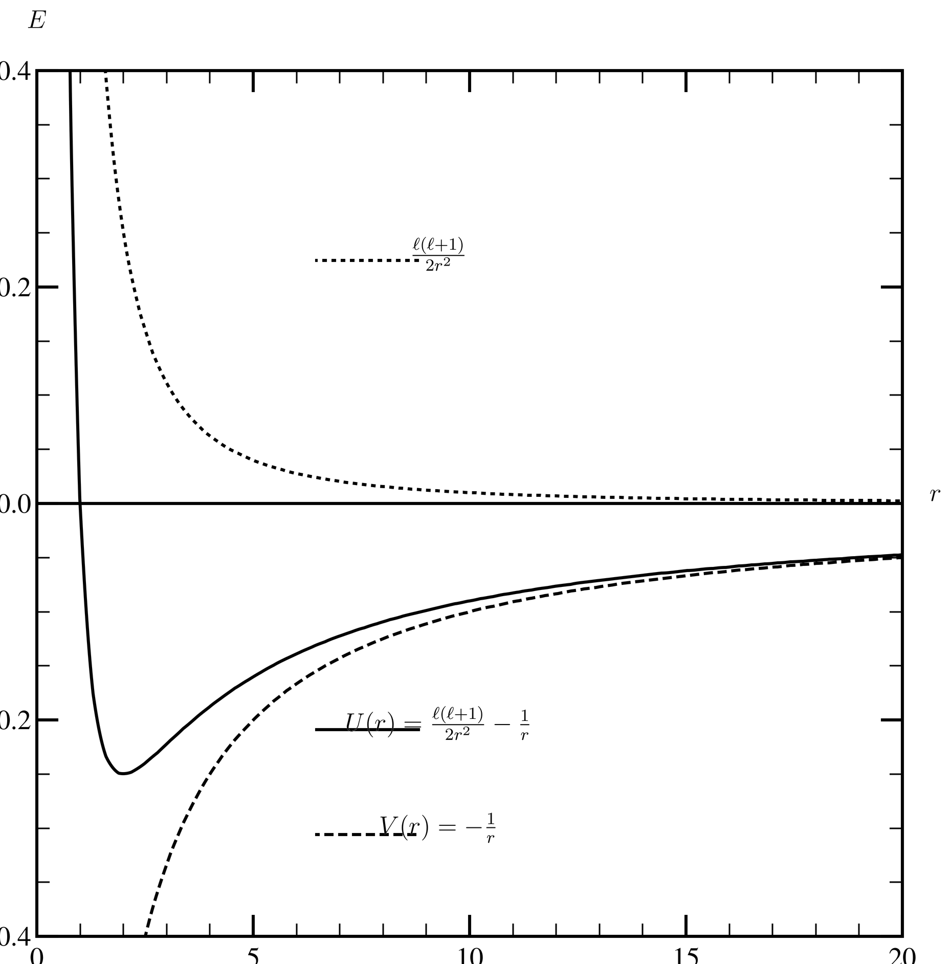
Figure 1:The true, centrifugal and effective potentials for hydrogen, for the case . Energy (vertical axis) and radius (horizontal axis) are measured in modified atomic units.
Returning to the radial Schr"odinger equation (5), we sketch the effective potential, as shown in Figure 1. The positive centrifugal potential dominates for small , while the negative true potential dominates for large . The competition between the two produces a well in the effective potential, as shown in the figure, and we can expect bound states. In fact, the well supports an infinite number of bound states, for all values of . This is because of the long tail, which dies off only as . One can see from the figure that there are also unbound states with energies in the range . We will be mainly interested in the bound states in this set of notes, but one must remember that there are also unbound states. In particular, a resolution of the identity requires both the bound states and unbounded states (the bound state wavefunctions by themselves do not form a complete set). See (114).
In modified atomic units, the radial Schr"odinger equation (5) becomes
To find the bound states (for which ) it is convenient to introduce a parameter
Next, to transform the radial wave equation to a standard form, we first define a modified radial variable,
whereupon (6) becomes
To obtain the asymptotic (large ) behavior of the solution , we neglect the terms in and , whereupon we find . The solution that goes as is not normalizable, so we want the one that goes as at large .
This leads us to define a new radial wave function by
where we have also removed a factor of to account for the behavior of at the origin (see Behavior of the Radial Eigenfunctions Near ) as well as the extra factor of connecting and [see (10)]. Substituting this into (6) gives an equation for ,
If we seek a power series solution for this equation, we find that if the power series does not terminate, then diverges as as , thereby overwhelming the factor in (10) and causing the solution to diverge. Such solutions are not normalizable and not acceptable as bound states. But we find that if is an integer , then the power series solution of (11) terminates, that is, it is a polynomial. In this case the wave function is normalizable, and we have a bound state solution. To represent these bound states, we will henceforth write instead of , where for given , takes on the values
The degree of the polynomial solution to (11) is . The integer is called the principal quantum number. Now (7) gives the energy as a function of ,
This is in modified atomic units; we must multiply by (see Table 2) to convert to ordinary units. We see that there are an infinite number of bound states for each value of .
(11) is a second order differential equation that must have two linearly independent solutions, of which the power series solution we have discussed in the preceding paragraph is only one. We should investigate the other solutions. To obtain them we use the method of Frobenius, in which one seeks a solution of the form,
that is, a power series multiplied by a fixed power, which, if negative or fractional, indicates a singularity at . In fact, plugging (14) into (11) shows that one solution has , which is the power series mentioned above; in that case the power series terminates if satisfies (12). The other solution has , which has a singularity at the origin. This solution leads the the small dependence of the radial wave function , which was discussed in general terms in Behavior of the Radial Eigenfunctions Near . That solution is nonphysical and is rejected. There remain only the polynomial solutions with .
The transformations leading up to (11) have put it into the standard form for the differential equation satisfied by the associated Laguerre polynomials. See Abramowitz and Stegun, Chapter~22, and table entry (22.6.15). Abramowitz and Stegun denote the associated Laguerre polynomials by ; they are polynomials of degree in , parameterized by (with reference to their notation, note that their is not the same as ours).
Writing out the standard differential equation for the Laguerre polynomials and comparing it to (11), we find the solution,
so that
where we have appended the quantum numbers to the radial wave function.
The Normalization
To normalize the radial wave functions we use the generating function of the associated Laguerre polynomials. This is a somewhat technical exercise, which we now outline. For the generating function, see Abramowitz and Stegun, table entry (22.9.15), which we write in the form
where we have changed the notation slightly to avoid conflict between our notation and that of Abramowitz and Stegun. Function is the generating function of the associated Laguerre polynomials, and (17) can be regarded as the definition of those polynomials. We write out (17) again, with and , and multiply both sides together. Then we multiply both sides by and integrate from to . On the left we obtain
while on the right we obtain
Expanding the left hand side (18) in a double power series in and and picking out the term in and equating it to the same term on the right, we find the integral,
This allows us to normalize the radial wave functions (16), where we set and . We write the result in terms of the version~1 radial wave function,
where we recall that and that the result is expressed in modified atomic units.
Now the orthonormality conditions for the radial wave functions are
Notice that the radial wavefunctions are orthonormal only for fixed ; there is no simple orthonormality condition connecting radial wave functions of different . The three-dimensional wave functions are orthogonal for different because of the orthogonality of the 's.
Beware in comparing these results to other authors (e.g., Schiff), who use different conventions for the associated Laguerre polynomials. Here we have followed Abramowitz and Stegun.
The generating function can also be used to compute expectation values of powers of , that is,
The process is somewhat lengthy and not very illuminating, however, and the calculation is somewhat different for every different value of . But if we do this for the special case , for which the answer is given by (38), then we can use the Kramers relation (see Prob.~\prbrhydrogen-1) to obtain for all other integer values of .
The Energy Levels
In central force problems the radial wave equation is parameterized by , so we get a different set of energy levels for each . It is often convenient to plot these on a diagram in which the levels for each value of are arranged in a column labeled by . Effectively this is a plot with energy on the vertical axis and angular momentum on the horizontal axis. Doing this for hydrogen, we obtain Figure 2.
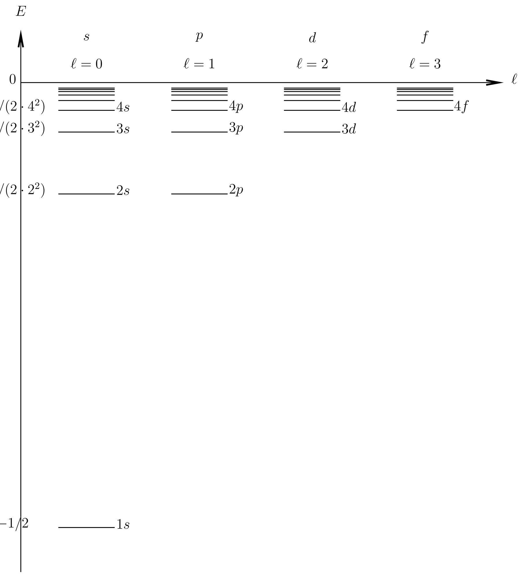
Figure 2:The energy levels of a hydrogen-like atom in the electrostatic model, with energy measured in modified atomic units.
As seen at the top of Figure 2, the angular momentum quantum numbers are associated with a series of code letters, , , , , etc. After the code letters follow the letters of the alphabet, , , , etc. These have only a historical significance, but they are used universally in spectroscopic notation so one must know them and how to translate them into angular momentum values. The energy along the vertical axis is given in in modified atomic units (see Table 2). The energy levels within a given column are sequenced by principal quantum number , which according to (12) begins with at the bottom of the column and increases by one at each successive higher level in the column. An infinite number of these levels accumulates below , which is the continuum threshold. The spectroscopic notation for a given level in a given column is , where is replaced by the one of the code letters, , , , , etc. For example, the ground state is denoted .
We can make a plot like this for any central force problem. Since the radial Schr"odinger equation is parameterized by , we get in effect a different spectrum for each value of . For a randomly chosen central force potential, these different spectra are effectively unrelated to one another, and there is very little chance that a level in one column will coincide with a level in another. At least, not exactly; of course they can come very close, and they will do so in regions where the energy levels are closely spaced. But an exact coincidence is unlikely.
A unique feature of hydrogen, however, is that there is an exact degeneracy among the levels of a given across the different columns. That is because the energies, given by (13), depend only on and are independent of . This degeneracy is not due to rotational invariance, which only explains why the energies are independent of the magnetic quantum number . Instead, it is due to the fact that hydrogen, in the electrostatic model, possesses a larger symmetry group than , the group of rotations, which is the symmetry of any central force problem. Hydrogen, as it turns out, has the symmetry group for the bound states, the group of proper rotations in a Euclidean space of four dimensions. These four dimensional rotations do not act solely on the configuration space coordinates of the hydrogen atom, that is, the , and coordinates of the electron; instead, they involve nontrivial transformations that affect both the position and the momentum of the electron. The generators of this symmetry include (which of course generates ordinary rotations) and the Runge-Lenz vector. We will not go into the details of this extra symmetry of the hydrogen atom, but a readable introduction to it is given by Schiff.
The total degeneracy of the energy level can be obtained by summing degeneracies horizontally across the levels of Figure 2. Each level shown in the figure is actually degenerate levels, because of the magnetic quantum number which runs over . Therefore the total degeneracy is
Breaking the Extra Degeneracy
As we have explained, the degeneracy between states of the same but different is not a general feature of central force potentials but rather is unique to hydrogen. Therefore any central force perturbation to the Coulomb potential will break the degeneracy in while maintaining that in . We now present two physically interesting ways of doing this.
One concerns is the volume effect, which is explored in detail in Prob. Paragraph. The volume effect is due to the fact that the nucleus is not a point charge, but rather has its charge spread out over a finite volume. This modifies the energy levels of the atom somewhat.
The radius of a proton or a neutron is roughly , and when nucleons are bound to one another in a compound nucleus they behave roughly like hard spheres in contact. Thus, a simple model of the nucleus is a sphere of radius , where is the total number of nucleons, over which the total charge is spread out in some manner. The charge density dies off rapidly outside the nuclear radius, so that well outside the nucleus the electrostatic potential is the Coulomb potential, . Inside the nucleus, however the true potential deviates significantly from the Coulomb potential, and, in particular, it does not diverge as .
Taking into account the spread in the nuclear charge, the potential is not exactly a Coulomb potential, so we should not expect to see an exact degeneracy in . But the nucleus is very small compared to an atom, for example, it is nearly 105 times smaller in the case of hydrogen. So the region over which the potential deviates from the Coulomb potential is relatively very small. Given the behavior of wave functions near the origin, as discussed in Behavior of the Radial Eigenfunctions Near , we can expect -waves (with ) to be most strongly affected by the volume effect. This is indeed the case; the states with higher values of are hardly affected. But overall, there is a dependence on introduced into energy levels, thereby breaking the -degeneracy of the pure Coulomb field.
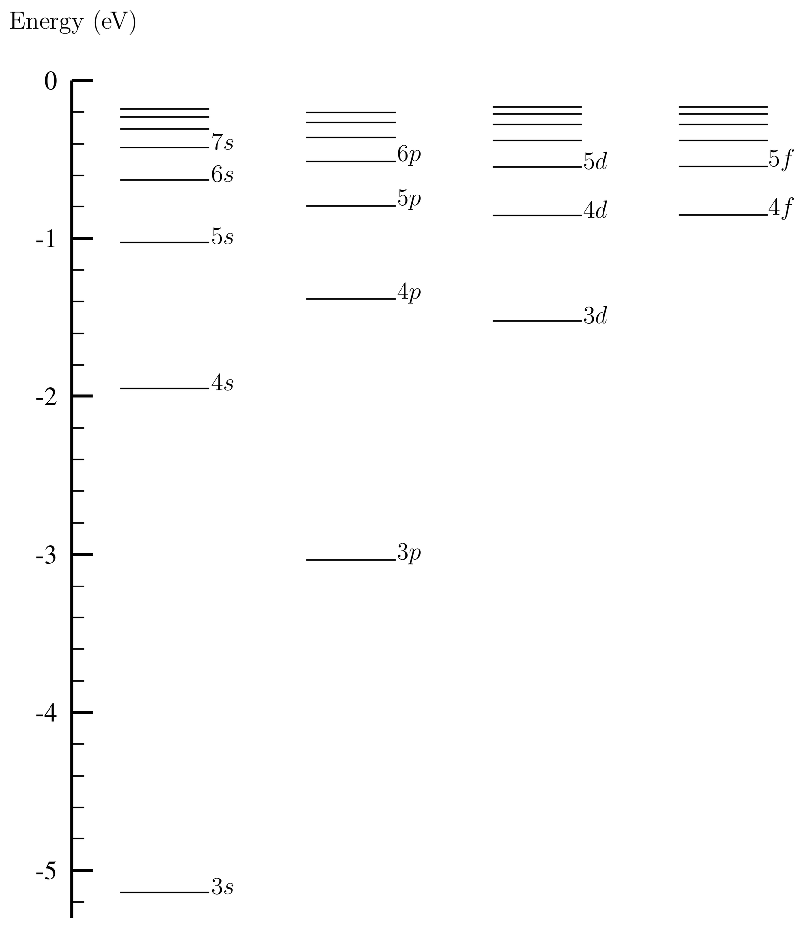
Figure 3:Energy level diagram for sodium (source: NIST database). Energy is the ionization limit for a single electron (one electron at infinity plus a ion in its ground state). Only the few lowest lying levels are shown. These illustrate the strong dependence of the energy on the quantum number .
Central Force Model of Alkali Atoms
The second example is a simple model of the alkali atoms. Neutral alkali atoms such as have one electron in the outer, valence shell, which surrounds a core of completely filled subshells containing electrons. A model of such atoms treats the inner core as a spherically symmetric distribution of negative charge that screens the nuclear charge. The amount of screening depends on the radius; as , the full, unscreened charge of the nucleus is seen, whereas when the valence electron is pulled far away from the core, it leaves behind an ion of +1 unit of charge. We can use Gauss’ law to find the electric field (which under our assumptions has only a radial component) seen by the valence electron,
where is the total charge inside radius . It has the limiting forms,
This gives the potential for the valence electron,
There is no simple formula for or for .
Like the Coulomb potential, the screened potential (27) goes to as , and to 0 as . But the manner in which it does so is not like any given Coulomb potential with a fixed , and if it is regarded as a perturbation of a Coulomb potential with a fixed , then the perturbation is not small. Thus, we should expect some strong breaking of the degeneracy in that is present in hydrogen-like atoms.
The energy level diagram for sodium, shown in Figure 3, shows that this is the case. In sodium the principal quantum number begins with because the two inner shells are filled. Notice that the level is not at all close to the level, in fact, the transition is the sodium -line, the strong yellow line that makes most fires yellow. It is an optical transition, with an energy comparable to transitions between states of different in hydrogen. Note, however, that the and levels of sodium are nearly degenerate. This is because when is large the classical orbit is nearly circular, so that if is large, too, then the electron’s orbit remains well outside the atomic core. Out in that region, the potential is approximately that of hydrogen. States of small , even when is large, involve orbits that dive into the core where the non-Coulomb nature of the potential is felt.
The Wave Functions
Returning to hydrogen, we can obtain an explicit formula for the Laguerre polynomials either by expanding the generating function (17) in powers of or by reference to Abramowitz and Stegun, table entry (22.3.9). This gives
From this we can work out the first few radial wave functions , which we tabulate here:
where we have restored ordinary units and , the effective Bohr radius, is given in Table 2. It is worthwhile mentioning that while the energies do not depend on the angular momentum quantum number , the wave functions depend on both and .
The method that has been used in these notes to derive the energy eigenvalues and eigenfunctions for hydrogen, that is, the method based on a power series expansion of the solution, can be used successfully in several problems in quantum mechanics. In addition to the hydrogen atom, problems solvable by this method include the harmonic oscillator, which leads to Hermite polynomials; the -equation in the theory of the spherical harmonics, which leads to the associated Legendre polynomials; the -matrices, which are the wave functions for the rotational motion of symmetric-top molecules, which lead to Jacobi polynomials; and several others. You will be aware, of course, that in the case of the harmonic oscillator (08. Harmonic Oscillators and Coherent States) and the 's (15. Orbital Angular Momentum and Spherical Harmonics) we did not rely mainly on differential equations or power series, rather we used algebraic techniques, that is, raising and lowering operators. It is natural to ask, therefore, whether algebraic techniques exist also for hydrogen. The answer is yes, and the method is tied up with the symmetry of the hydrogen atom mentioned earlier. In these notes we have chosen to use more traditional methods to solve the hydrogen atom, because it would take us too far afield to develop the algebraic techniques.
We will mention, however, that the algebraic techniques in question involve a mapping from the bound states of hydrogen onto the spherical harmonics in four dimensions, that is, the harmonics that live on the 3-dimensional surface of a sphere in 4-dimensional, Euclidean space. The symmetry group acts on this sphere by 4-dimensional, orthogonal transformations. As for the unbound states of hydrogen with , these correspond to harmonics on the unit mass hyperboloid in 4-dimensional Minkowski space. For these the symmetry group is , that is, the Lorentz group. The appearance of the Lorentz group here has nothing to do with relativity in a physical sense, it is just that the mathematics of the positive energy solutions of hydrogen gives rise to it.
Problems
Problem 1.
This problem involves some exercise with expectation values of powers of in hy-dro-gen-like atoms. These expectation values are useful in perturbation theory and other places. There are various ways to evaluate these expectation values; for example, one can use the generating function of the Laguerre polynomials. But I think the following method is somewhat easier, once you get it going.
(a) Write out the radial Schr"odinger equation for a hydrogen-like atom. (“Hydrogen-like” means .) Show that if , then
where is the normalized radial wave function corresponding to quantum numbers and . Now multiply this by and integrate from 0 to . Use integration by parts to show that
In the integrations, you may assume that , which will cause the boundary terms to vanish.
(b) Now multiply (35) by and do more integration by parts, and combine the result with (36) to show that
This is called the Kramer’s relation.
(c) Use (37) to find for , , and . Notice that you cannot evaluate by this method. For that you need to face up to generating functions, or some other method. However, given that
find . The latter is needed for the fine structure perturbations and the Zeeman effect.
Problem 2.
Look up the energies of the and levels of sodium on the NIST data base, and compare to the theoretical energy of the level of hydrogen. You will see that some of the levels of sodium are actually close doublets; this is the fine structure, which does not appear in Fig.~\figr\cn.3 because it is too small on the scale of the figure.