23. Bound-State Perturbation Theory
Introduction
Bound state perturbation theory applies to the bound states of perturbed systems, for which the energy levels are discrete and separated from one another. The system may also have a continuous spectrum, but the interest is attached to the discrete states. The effects of perturbations on states of the continuous spectrum, or on discrete states imbedded in the continuum, require different techniques, such as time-dependent perturbation theory.
The version of bound-state perturbation theory that you are probably familiar with is called Rayleigh-Schr"odinger perturbation theory. In these notes, we will begin with a variation on Rayleigh-Schr"odinger perturbation theory, called Brillouin-Wigner perturbation theory. The Brillouin-Wigner theory is simpler and less messy to derive than the Rayleigh-Schr"odinger theory, and it also gives more accurate answers in many circumstances. Its disadvantage is that the unknown energy levels are given only implicitly, in terms of the solutions of nonlinear equations. But if explicit formulas for the energy levels are desired, it is easy to expand the solutions in powers of the perturbation parameter, whereupon the results of the Rayleigh-Schr"odinger theory are recovered. In my opinion, this is the easiest and most elegant way to derive Rayleigh-Schr"odinger perturbation theory.
The Unperturbed and Perturbed States
We consider an unperturbed Hamiltonian with eigenvalues and eigenstates , where is an index introduced to resolve degeneracies, so that
See Figure 1, in which the unperturbed levels are illustrated on a vertical axis. Although we use a notation appropriate for a discrete spectrum of , we actually allow it to have a mixed spectrum, typically a continuous spectrum above some energy and a discrete one below that, as often happens in practice. Sums over states, such as (4), must be interpreted as including the continuous part of the spectrum, as necessary, as shown for example in (113) and (114).
We pick one of the discrete levels for study, so the index will be fixed for the following discussion. We denote the eigenspace of the unperturbed system corresponding to eigenvalue by , so that the unperturbed eigenkets form a basis in this space.
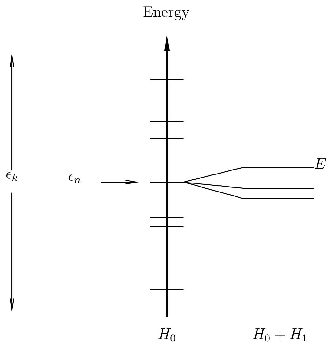
Figure 1:The energy levels of the unperturbed system are shown on a vertical axis. These levels are degenerate in general. One of these, , is selected out for study. When the perturbation is turned on, level may split and shift. The energy level of the perturbed system is one that grows out of as the perturbation is turned on.
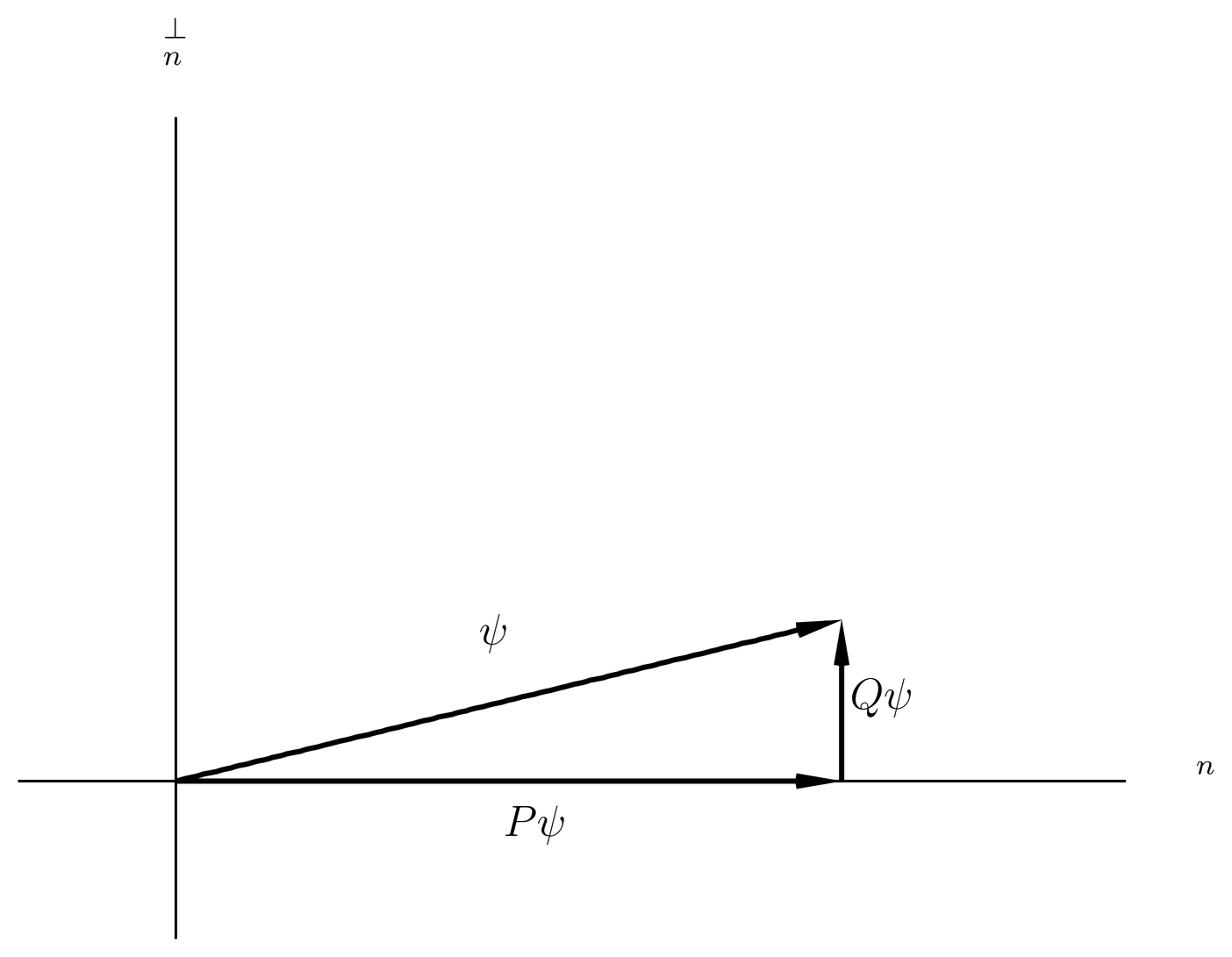
Figure 2:Subspace is the unperturbed eigenspace for level , and is the orthogonal subspace. Projectors and project onto and , respectively. The exact eigenstate lies approximately in , with a small correction orthogonal to this subspace.
We take the perturbed Hamiltonian to be , where is a formal expansion parameter that we allow to vary between 0 and 1 to interpolate between the unperturbed and perturbed system. When the perturbation is turned on, the unperturbed energy level may split and shift. We denote one of the exact energy levels that grows out of by , as shown in Figure 1. We let be an exact energy eigenket corresponding to energy , so that
Both and are understood to be functions of ; as , approaches and approaches some state lying in . (2) only determines to within a normalization and phase, which can be functions of ; we are free to choose as we wish these to simplify our work.
It helps to have a picture of the perturbation problem in terms of the geometry of Hilbert space. We break the Hilbert space into the subspace and its orthogonal complement which we denote by . The latter space is spanned by the unperturbed eigenkets for all . Since the perturbation is small, the exact eigenket presumably lies nearly in , with only a small component orthogonal to , as illustrated in Figure 2. The components of parallel and perpendicular to are conveniently expressed in terms of the projector onto the subspace and the orthogonal projector , defined by
and
These projectors satisfy , , and . They also commute with ,
since they project onto eigenspaces of . In terms of these projectors, the components of parallel and perpendicular to are and , respectively, as illustrated in Figure 2.
The component of the exact eigenstate lies in the unperturbed eigenspace, and thus is itself an unperturbed eigenstate. It is therefore a linear combination of the known unperturbed eigenstates . The orthogonal component , on the other hand, is harder to find. In the following we will think of as the easy part of and as the hard part, and attempt to solve for the hard part (or else the total solution ) in terms of the easy part . It turns out it is possible to write a neat power series expansion for this solution, (17) below.
As a first step in the derivation of this series, we rearrange (2) in the form,
We would like to divide this equation by to solve for , but before proceeding we must examine to see if it is well behaved. The idea of dividing by is closely related to the use of Green’s functions. See 37. Green’s Functions in Quantum Mechanics, where the basic idea is presented and developed.
The Inverse of on 
The operator is a function of the operator , which according to (133) can be written in terms of the eigenvalues and projectors of ,
The resulting expression, however, is meaningless if the exact eigenvalue should equal any of the unperturbed eigenvalues . In that case, one or more denominators vanish, indicating that does not possess an inverse. Even if none of the denominators vanishes, nevertheless the exact eigenvalue is presumably close to the unperturbed eigenvalue , and therefore the terms in (7) are large (and these terms diverge at , where ).
In order to avoid small or vanishing denominators, and to work with operators that are guaranteed to be well defined, we define a new operator which is (7) with the terms suppressed:
The operator is closely related to the Green’s operators that we shall consider later in the course, when we take up scattering theory.
It is possible that is not the only small or vanishing denominator in (7). For example, if there are other unperturbed energy levels lying close to , then the perturbation could push the exact energy near to or past some of these other levels, and then other small denominators would result in (7). This will certainly happen if the perturbation is large enough. For the time being we will assume this does not happen, so that (8) is free of small denominators. This is the situation illustrated in Figure 1. When this is not the case we shall refer to “nearly degenerate perturbation theory,” which is discussed in Nearly Degenerate Perturbation Theory.
The operator satisfies
and
These equations show that vanishes on the subspace , while it is the inverse of on the subspace . Note that is just the identity operator on .
A series for in terms of 
We return now to (6) and multiply through by , using (10). This gives
which expresses the “hard” part of the exact eigenstate in terms of the total exact eigenstate . To turn this into something more useful, we first add to both sides, obtaining
This expresses the exact eigenket in terms of its projections onto and , of which the second term is a small correction. It is not an explicit solution for since occurs on the right hand side, but it can be converted into a power series solution by a method of successive approximation.
In particular, note that if we neglect the second term in (12), which is of order , we obtain , which is correct to lowest order. To improve on the approximation, we substitute the left hand side of (12) into the second term on the right hand side, obtaining,
which is still an exact equation. Now all terms on the right hand side except the last one involve the “easy” part of the exact eigenstate, and only the final term, which is second order in the perturbation, involves . If we neglect that term, we obtain an expression for in terms of that is valid to first order in . Continuing this way, we can substitute the left hand side of (12) into the last term in (13), to push the hard term to fourth order in , etc. The result is a formal power series for the solution in terms of the easy part .
Another way to get the same thing is to rearrange (12),
so that
The inverse operator is then easily expanded in a series,
This is the basic series out of which all the results of perturbation theory are constructed. The series might not converge, but in perturbation theory we do not necessarily need convergent series.
Nondegenerate Perturbation Theory
In nondegenerate perturbation theory the level of is nondegenerate. Then the index is not needed for the level , and we can write simply for the corresponding eigenstate. We retain for the other levels , since these may still be degenerate. Then since the space is 1-dimensional and is spanned by , we must have , where is some constant. It is obvious from Figure 2 that and cannot both be normalized, since one is the base and the other the hypotenuse of a right triangle. In the following it is convenient to choose the normalization and phase of so that . Thus we have
where we assume that and the other unperturbed eigenstates are normalized. This is the most convenient normalization convention for nondegenerate perturbation theory, but it means that is not normalized, in fact from Figure 2 it is clear that , since the hypoteneuse is longer than the base. After we are done with the perturbation expansion, we are free to normalize in the usual way. With this normalization convention, we have
Now the series (17) becomes
which expresses the exact eigenket as an infinite series in terms of the unperturbed eigenket . However, the operator still involves the unknown energy level , which appears in the denominators, so (22) is still not an explicit solution for the exact eigenket .
To find an equation for , we multiply (6) on the left by and use (19) to get
and then we substitute (22) into this. Thus we find
Since the unknown exact energy still appears in the denominators on the right hand side of this equation, this is not an explicit solution for . But (25) does give explicitly through ,
which agrees with the usual result of Rayleigh-Schr"odinger perturbation theory. If we want the energy correct through , we can substitute the zeroth order approximation for , namely, , into the denominator of the term in (25), whereupon we find
which agrees with Rayleigh-Schr"odinger theory through . Similarly, if we wish the energy correct to , we can substitute the first order expression (26) for into the denominator of the term in (25), and the zeroth order expression into the term, etc. When the denominators are expanded out in powers of , the results of Rayleigh-Schr"odinger perturbation theory are recovered. At third order and beyond, the expressions of the Raleigh-Schr"odinger theory are more complicated than those of the Brillouin-Wigner theory, because of the extra terms that come from expanding the denominators.
Once the energy has been determined in this manner, we can go back to (22) and obtain the eigenkets. For example, through first order we have
which again is the usual result from Rayleigh-Schr"odinger perturbation theory.
Degenerate Perturbation Theory
In the case that the unperturbed energy level is degenerate, the projection of the exact eigenket onto must be a linear combination of the unperturbed eigenkets ,
where are the expansion coefficients. Since is orthogonal to all the kets , we have
To obtain an equation for the ’s, we multiply (6) on the left by and use (30) to obtain,
We substitute (17) into this, using (29) for , and we find
This equation must be solved simultaneously for the eigenvalues and the unknown expansion coefficients .
We see that the expansion coefficients , which determine by (29), are the eigenvectors of a matrix, where is the degeneracy of the unperturbed eigenvalue , and that the energy shifts are the eigenvalues. But this is not the standard problem of determining the eigenvalues and eigenvectors of a matrix, because the unknown energies appear not only on the left-hand side but also in the denominators in the second and higher order terms of the matrix.
In practice, however, the most common type of problem is one in which we desire the energy shifts to first order in . We can find these by truncating the series in (33) at first order, whereupon the energy shifts are the eigenvalues of the matrix , that is, they are the eigenvalues of the matrix of the perturbing Hamiltonian inside the degenerate eigenspace of unperturbed system. At this order there are no energy denominators to worry about and we can just diagonalize the matrix. Also, the eigenvectors corresponding to the energy shifts determine via (29), so that the perturbed eigenkets are known to zeroth order. In many applications this is sufficient (see, for example, the treatmant of the Stark effect on the levels of hydrogen in The Perturbed Eigenfunctions).
The first order matrix may or may not have degeneracies itself. If it does not, then all degeneracies are lifted at first order; if it does, the remaining degeneracies may be lifted at a higher order, or may persist to all orders. Degeneracies that persist to all orders are almost always due to some symmetry of the system, which can usually be recognized at the outset.
To proceed to second order, we may substitute the zeroth order solution into the denominators of the second order term in (33) and truncate the series at this order. We then obtain a new eigenvalue-eigenvector problem for the unknown energy corrections and coefficients , which differs from the one we had at first order by the addition of a second order matrix as a correction to the matrix that we had at first order. We can evaluate the eigenvalues and eigenvectors of the sum of these two matrices by standard matrix techniques, or we can regard the new eigenvalue-eigenvector problem as a new problem in bound state perturbation theory, in which the first order matrix plays the role of a new unperturbed Hamiltonian, say, , and the second order matrix plays the role of a new perturbation, say, . We will have to use either the nondegenerate or degenerate versions of this theory, depending on whether or not all degeneracies of the original Hamiltonian were lifted at first order. In any case, once the energies and coefficients have been determined to some order, they can be substituted into (29) to determine .
Finally, once and are known to some order, these can be substituted into (17) to determine .
Nearly Degenerate Perturbation Theory
Now let us consider the case in which the unperturbed levels of , while not technically degenerate, are close to one another. This often happens in practice, because levels are often grouped into multiplets of closely spaced levels, which are more widely separated from other multiplets. Suppose to be specific that two levels, say, and , are close enough to one another that first order perturbations will push the exact level close to or onto the unperturbed level . Then the denominators in the terms in (8) are small, and that equation cannot be used.
In this case we may proceed as follows. Let us choose choose some energy, call it , which is close to and . It could, for example, be one of the energies or themselves, or it could be their average, etc. Then let us take the original unperturbed Hamiltonian and perturbation and rearrange them in the form,
where
In effect, we have merged the nearly degenerate levels , into a single degenerate level , and thrown the correction terms into . Then standard degenerate perturbation theory may be applied. We will call this procedure “nearly degenerate perturbation theory.”
An equivalent approach to nearly degenerate perturbation theory is to exclude both sets of terms and from the definition of , and to proceed from there. Then becomes the inverse of on the space orthogonal to .
Problems
Problem 1.
This problem concerns the volume effect, which was discussed briefly in Sec.~\secr\hydrogen.8.
(a) Compute the shifts in the energy levels of a single-electron (hydrogen-like) atom of nuclear charge due to the finite size of the nucleus. Treat the nucleus as a uniform sphere of charge of radius , where cm and is the number of nucleons. Express your answer as some number of eV times some function of , , and the quantum numbers of the atomic state. Only treat those atomic states for which the effect is the largest. This is called the volume effect. You may use
valid in hydrogen-like atoms, where is the Bohr radius.
The volume effect induces a splitting between the and levels of hydrogen. Compare this to the Lamb shift (another splitting of the same two levels). The Lamb shift raises the level relative to the level by approximately 1.05 GHz in frequency units.
(b) A muonic atom is one in which the electron has been replaced by a negative muon , a particle with a charge and a mass of 105~. Compute for the volume effect via first order perturbation theory for the level of muonic uranium (). Is this calculation reliable?
Problem 2.
In this problem, set for simplicity. The Hamiltonian for a rigid body is
where are the principal moments of inertia and where are angular momentum operators satisfying the commutation relations,
You may assume that the angular momentum takes on only integer values. The Hamiltonian (38) describes the rotational spectrum of molecules. Physically, the quantities are the negatives of the components of the angular momentum with respect to the body frame.
In the case of a spherical top, such as methane (), we have . The Hamiltonian is
and the energy levels are
which is -fold degenerate since is independent of .
In the case of a symmetric top such as ammonia(), we have . The Hamiltonian is
and the energy levels are
where
and where is the usual quantum number of .
Now consider the case of a slightly asymmetric top. (Water is an example of an asymmetric top molecule.) Let
where is small. These equations are equivalent to defining
Write the Hamiltonian as , where is the symmetric top Hamiltonian in (42).
You may find the following relations useful:
but if you use (48) you must prove it.
(a) Consider the state . Find the first order of perturbation theory at which the energy shift does not vanish, and compute the energy shift at that order. In addition to the abbreviations (44), use
and express your answer in terms of the constants , and .
(b) Find the first order of perturbation theory at which the energy shifts for the levels do not vanish, and compute them at that order.
(c) Find the first order of perturbation theory at which the energy shifts for the levels do not vanish, and compute them at that order. Express your answer in terms of
Notice the appearance of a sum over “intermediate states.”
(d) What order of perturbation theory do you have to go to in order to find the first nonvanishing correction to the energy in the case of ? ?