14. Spins in Magnetic Fields
Introduction
A nice illustration of rotation operator methods that is also important physically is the problem of spins in magnetic fields. The earliest experiments along these lines were those of Stern and Gerlach, which in 1922 first revealed the quantization of electron spin. Similar but later experiments by Stern and other collaborators were used to make crude measurements of the proton magnetic moment and other nuclear magnetic moments. In the 1930’s Rabi developed the techniques of spin flipping with time-dependent magnetic fields, which he used to make much more accurate measurements of nuclear magnetic moments as well as important discoveries such as the existence of an electric quadrupole moment in the deuteron. After World War II, Bloch and Purcell developed methods for studying magnetic resonance in bulk samples (solid or liquid), by measuring microwave power absorbed at resonance or by looking at the time development and relaxation of induced magnetization. In the same period, Rabi’s beam techniques were improved upon by Ramsey and Hahn developed the method of spin echo, in which the dephasing of a bulk magnetization is time-reversed following a spin flip and the original magnetization is restored. The spin echo technique now forms the basis of medical imaging by magnetic resonance. Modern applications of magnetic resonance include measurements of nuclear magnetic moments and -factors, measurements of diamagnetic shielding of external fields in molecules or solids (important in chemistry and solid state physics), the construction of sensitive magnetometers and atomic clocks, and tomography or imaging in medicine and biology.
Earlier in the course we examined experimental and gedanken-experimental data from the Stern-Gerlach experiment, which concerned the measurement of the magnetic moment of silver atoms. In these notes we will focus on the magnetic moments of a variety of particles, including elementary particles such as the electron and muon and well as composite particles such as nucleons (protons and neutrons), nuclei themselves, atoms and molecules. The existence of a magnetic moment, a vector of observables, implies that there is a kind of internal, orientational degree of freedom to such particles. This degree of freedom is associated with what we call the “spin” of the particle, which is the generator of rotations on the Hilbert space describing these internal degrees of freedom.
Magnetic Moments and Angular Momentum
We begin by reviewing magnetic moments in classical electromagnetism. Consider a localized current distribution . (This is the electric current, not to be confused with an angular momentum.) You may think of the currents that are present in an atom or nucleus. Associated with this current distribution is the magnetic moment, defined by
Here we write the variable of integration as , which runs over the current distribution, to distinguish it from field points to be introduced momentarily. Since is integrated over, the magnetic moment does not depend on position , but it may depend on time.
If the current distribution is placed in an external magnetic field then it experiences a force and a torque given by
These expressions are derived in books on electromagnetism, such as Jackson, Classical Electrodynamics. They are based on the approximation that the magnetic field is slowly varying over the extent of the current distribution, something that for laboratory scale magnetic fields and dipoles of atomic or nuclear size would be an excellent approximation. Note that in (2) the gradient operator only acts on , since is independent of . The current distribution is presumably produced by charged particles. If the force (2) is the only force acting on the system and if above is chosen to be the center of mass then by Newton’s laws we obtain an equation of motion for the center of mass of the system,
and another for the angular momentum of the system about the center of mass,
Equation (4) normally applies to a system that is electrically neutral, such as a neutron or a silver atom; if the system has a net charge then there will also be the Lorentz force and possibly an electric force .
We cannot solve (4) for the trajectory of the center of mass without knowing how depends on time. Thus, we also need an equation for the time dependence of . (5) is not that, unless we have a relation between and .
In some circumstances is proportional to , in fact, such a proportionality is implied by the Stern-Gerlach results analyzed in 02. The Postulates of Quantum Mechanics. Those results, combined with a further analysis of signs and phase conventions [see (26) and \spatialdof.16], show that for a silver atom
where are the Pauli matrices and is a constant of dimensions of magnetic moment that can be determined experimentally. In fact, Stern and Gerlach measured , obtaining a value close to the Bohr magneton, a unit of magnetic moment given by
On the other hand, our analysis in 12. Rotations in Quantum Mechanics, and Rotations of Spin-1/2 Systems{} of rotations and angular momentum for spin- systems showed that , where now we write for the angular momentum instead of the general notation used in (25). Combined with (6) this shows that for a silver atom,
This relation actually describes the electron, since a silver atom acquires both its magnetic moment and angular momentum from its single, unpaired valence electron.
At this point it is instructive to consider a simple classical model of magnetic moment and angular momentum. Consider, for example, a particle of mass , charge , position and velocity in a circular orbit of radius . Placing the orbit in the - plane, the angular momentum is
while according to (1) the magnetic moment is
These imply
so that in this simple classical model, the magnetic moment and angular momentum are proportional.
They are not proportional in all classical models of mass and charge motion, however. This is easy to see, since the angular momentum depends on the mass distribution and its state of motion, while the magnetic moment depends on the charge distribution and its state of motion. These two do not have to be the same, for example, in a wire the electrons move and the ions are stationary. Thus, in classical mechanics and generally point in different directions. This question is explored in more detail in Prob.~\prbrspinmagf-4.
If we try to apply the classical equation (11) to the case of an electron, setting and and replacing by , we obtain (8), except for a factor of 2. Therefore in circumstances in which the angular momentum of a particle (which we call “spin”) is proportional to the magnetic moment, we can write the proportionality between them as
where is the charge of the particle, its mass and is the dimensionless, so-called -factor of the particle. The -factor is a fudge factor that hides our ignorance of how the magnetic moment is actually generated inside the particle.
For particles such as the electron, proton, neutron and atomic nuclei the magnetic moment is proportional to the spin and nontrivial -factors are required to express the proportionality quantitatively. Thus the question arises as to why these two vectors are proportional in these important cases, whereas classically they are not required to be so. This question cannot be answered at this point in the course but is addressed in Prob. Paragraph.
sec-spinmagf-3. The Hilbert Space for Spin and Magnetic Moments}
In the case of the silver atom we decided in 02. The Postulates of Quantum Mechanics{} that the Hilbert space upon which the magnetic moment operator acts is 2-dimensional, and that it is spanned by eigenkets of that we denoted by and :
Since is proportional to this is actually a standard angular momentum basis, one that we can also write as
where is the quantum number of the operator which has the eigenvalue (so that replaces in the general notation of 13. Representations of the Angular Momentum Operators and Rotations). As required by the angular momentum commutation relations, the quantum number belongs to the set shown in (33); only the one value is needed for this application, and it occurs with multiplicty 1, so the extra index seen in the general notation is not needed (see Degeneracies and Multiplicities). The Hilbert space consists of a single irreducible subspace under rotations, with .
It turns out that for other particles in the same class mentioned previously, including the electron, proton, neutron and atomic nuclei, the Hilbert space upon which the magnetic moment acts is also a single irreducible subspace under rotations whose value is what we call the spin of the particle. The Hilbert space and its standard angular momentum basis are described by
where is a fixed number belonging to the set (33), which like the -factor is a characteristic of the particle. Note that .
Thus another question arises, namely, why does the Hilbert space associated with the magnetic moment of these important particles consist of a single irreducible subspace under rotations? This question also cannot be answered at this point in the course, but the topic is addressed in Secs. Energy Eigenstates in Isolated Systems--The Nucleus and the M"ossbauer Effect. It turns out that the answer is related to that of the previous question, why the magnetic moment and angular momentum are proportional.
For the rest of these notes, we will accept that and are proportional and related by an equation such as (12), and that the Hilbert space is given by (15). This is all we need to talk about the spins and -factors of various particles.
Examples of Magnetic Moments and -factors
Let us look at some important examples of spins and magnetic moments. The data is summarized in Table 1.
Table 1:Spins and -factors for various particles and nuclei.
Particle | charge | spin | -factor |
|---|---|---|---|
electron | |||
positron | |||
proton | |||
neutron | 0 | ||
deuteron | 1 | ||
-particle | 0 |
For the electron, a spin- particle with , the relation (12) can be written
where and are the electron mass and -factor, and where we have multiplied and divided by to make the factor dimensionless. The factor is also dimensionless, so the quantity in the parentheses has dimensions of magnetic moment. This is the Bohr magneton, introduced in (7). The Bohr magneton is a convenient unit of magnetic moment for electrons or atoms with unpaired electrons.
The electron -factor can be written,
where the series indicated is a power series in the fine structure constant,
This series is the result of a perturbation calculation in quantum electrodynamics, in which the correction terms and higher are known as radiative corrections since physically they come from the interaction of the electron with the quantized electromagnetic and electron-positron fields. The first correction term in this series, shown in (17), was calculated by Schwinger in the late 1940’s, and was notable as one of the first successful applications of renormalization theory. These correction terms are small, so to a good approximation . The value comes out of the Dirac equation (the equation of the electron in relativistic quantum mechanics, see 46. Introduction to the Dirac Equation), so it is known as the Dirac value. For a time in the early days of atomic physics the existence of the small corrections was not known, either experimentally or theoretically, and it was believed that the -factor was exactly 2, as predicted by the Dirac equation. The discovery of the small deviations from the Dirac value led to a theoretical push to understand radiative corrections.
The discovery of radiative corrections has led to a competition between theory and experiment, to see if a discrepancy develops as the -factor is measured and calculated to ever higher precision. The purpose originally was to test QED, and now it has shifted to to a search for new physics, especially physics beyond the standard model. The -factor of the electron and other particles such as the muon are now among the most accurately known physical quantities.
Approximating the -factor by 2, the electron magnetic moment can be written,
The minus sign in this equation means that the electron magnetic moment and angular momentum point in opposite directions.
The positron is the antiparticle of the electron, with the same mass and -factor but opposite charge. Its magnetic moment is therefore given by
For the proton we have and , so
where the quantity in parentheses is the nuclear magneton,
so we can write
The nuclear magneton is a convenient unit for the magnetic moments of the proton, neutron and other hadrons and various nuclei. It differs from the Bohr magneton by the presence of the proton mass in the denominator instead of the electron mass, and so is about 2000 times smaller than the Bohr magneton. Nuclear magnetic moments, which are of the order of a nuclear magneton, are therefore much smaller than electron magnetic moments, so they make only small corrections to the total magnetic moment of an atom with unpaired electrons. If all the electrons in an atom are paired so that their magnetic moments cancel, then the nuclear magnetic moment is all that remains. The proton -factor is determined experimentally [see S.~G.~Karshenboim and V.~Ivanov, Phys. Lett. B 566, 27(2003)].
The neutron is electrically neutral, , but nevertheless has a nonzero magnetic moment given by
where . The neutron is considered to have a negative -factor, because and are in opposite directions. The usual electronic charge is used in , even though the neutron is neutral; and by convention, the proton mass is used in , even in the neutron equation (24). Crude models of mixtures of up and down quarks are able to explain the proton and neutron magnetic moments to within several percent, but it is very difficult to improve on these calculations. The difficulty is the usual one in hadron physics, where the strong interactions usually preclude a perturbative treatment.
The proton and neutron -factors are sometimes said to be anomalous, because they differ from the Dirac value of 2. Of course, so does the electron -factor, if we include the radiative corrections.
Nuclei have a variety of spins and magnetic moments. For the deuteron, a spin-one particle, we have
where . Notice that is the vector of matrices for spin 1, not the Pauli matrices (see (54) and (55)).
The magnetic moment of the deuteron can be considered as due to the magnetic moments of the constituent proton and neutron, plus some contribution due to the orbital motion of the proton. See Prob. Paragraph. Plugging in the actual numbers gives information about the deuteron wave function, that is, the wave function of the two particle system consisting of proton and neutron. More information about this wave function comes from scattering experiments, the measured electric quadrupole moment of the deuteron, and other sources. It turns out that the interaction between the proton and neutron is not governed by a purely central force potential, but rather there are strong spin-dependent forces as well. As a result, the spatial part of the wave function is not a pure eigenstate of orbital angular momentum, but rather consists of a linear combination of an -wave and a -wave (with and ). The deuteron has spin 1 because the energy of the proton-neutron system is minimized when the spins are aligned. When the spins are opposite, the proton-neutron system has no bound state. In fact, deuteron has no bound excited states (there is only one bound state, the ground state).
For the -particle, a spin-0 particle, we have exactly. Spin-0 particles cannot have a magnetic moment, because the spin operator vanishes [see (57)].
Hamiltonian for a Spin in a Magnetic Field
The force on a magnetic dipole (2) can be written as , where
that is, the quantity behaves as a potential energy, insofar as the total force on the dipole is concerned. Moreover, this quantity is also the energy of orientation of the magnetic dipole in an external magnetic field, as is shown in books on electromagnetism. Therefore it is a good guess that the Hamiltonian describing the motion of a neutral magnetic dipole in a magnetic field should be
If this is interpreted as a classical Hamiltonian, then by Hamilton’s equations it gives (4) for the acceleration of the dipole.
If the Hamiltonian (27) is interpreted as a quantum Hamiltonian, then it can be shown that it explains the splitting of the beam in a Stern-Gerlach apparatus. This requires techniques from adiabatic theory (see 39. Adiabatic Invariance, the Geometric Phase, and the Born-Oppenheimer Approximation), which we will not go into here.
For the rest of these notes we will restrict consideration to problems in which the magnetic field is uniform in space, so there is no coupling to the spatial degrees of freedom. This is often a good approximation in practice, since laboratory magnetic fields are usually quite uniform on the atomic scale. We will, however, allow the magnetic field to be a function of time, , because this in fact is the principal means by which spins are controlled experimentally.
As a result, we can ignore the spatial degrees of freedom and take the Hamiltonian to be
where
To be specific, in the rest of these notes we will assume (as it would be for an electron), but if then directions of precession and various other conclusions must be reversed.
The Time Evolution is a Rotation
Consider first the general problem in which the magnetic field has an arbitrary time dependence, . We denote the unitary time evolution operator by , reserving the symbol for rotation operators, as in 13. Representations of the Angular Momentum Operators and Rotations. The Schr"odinger equation for is (13), which in the present case is
If nothing further is said about the time dependence of , we cannot write down the solution in explicit form, but we can at least note that the time-evolution operator is always a rotation operator. To see this, we consider the infinitesimal time advance implied by the Schr"odinger equation,
The factor in the square brackets is an infinitesimal rotation operator, as we can see if we compare it to
valid when . We see that the axis of the infinitesimal rotation is given by
where we write
for the magnitude and direction of the magnetic field. The angle of the infinitesimal rotation is given by
or,
The angular velocity can also be written as a vector,
which is parallel to (antiparallel, if ).
We see that as time proceeds, develops by the composition of a large number of infinitesimal rotation operators; since the product of rotation operators is always a rotation operator, itself is a rotation operator. However, the axis and rate of rotation are in general functions of time. This is very much as in classical rigid body motion, in which is some function of time, which in general is not constant either in magnitude or direction. In classical rigid body motion, is determined as a function of time by solving the Euler equations; in the quantum mechanical motion of a charged particle in a magnetic field, is simply given as a function of time by (37). In either case, once is known, the subsequent problem of determining the time-dependent rotation is very similar.
Constant Magnetic Field
We turn now to some cases in which (30) can be solved explicitly. The simplest one is that of a spin in a constant magnetic field,
The Hamiltonian is now time-independent, so only depends on the elapsed time . We borrow notation from The Time Evolution is a Rotation, writing,
and
where now and its magnitude are time-independent. Thus the Schr"odinger equation for is
This can be immediately integrated, giving
The time evolution consists of a rotation about the axis with frequency .
In the case of the electron, the frequency of spin precession is
which, in the approximation , is equal to the nonrelativistic frequency of orbital motion of the electron in the uniform magnetic field (the gyrofrequency, see 10. Charged Particles in Magnetic Fields). Certain so-called experiments exploit this near equality to measure the small difference between the two frequencies, which provides a direct measurement of the radiative corrections in (17).
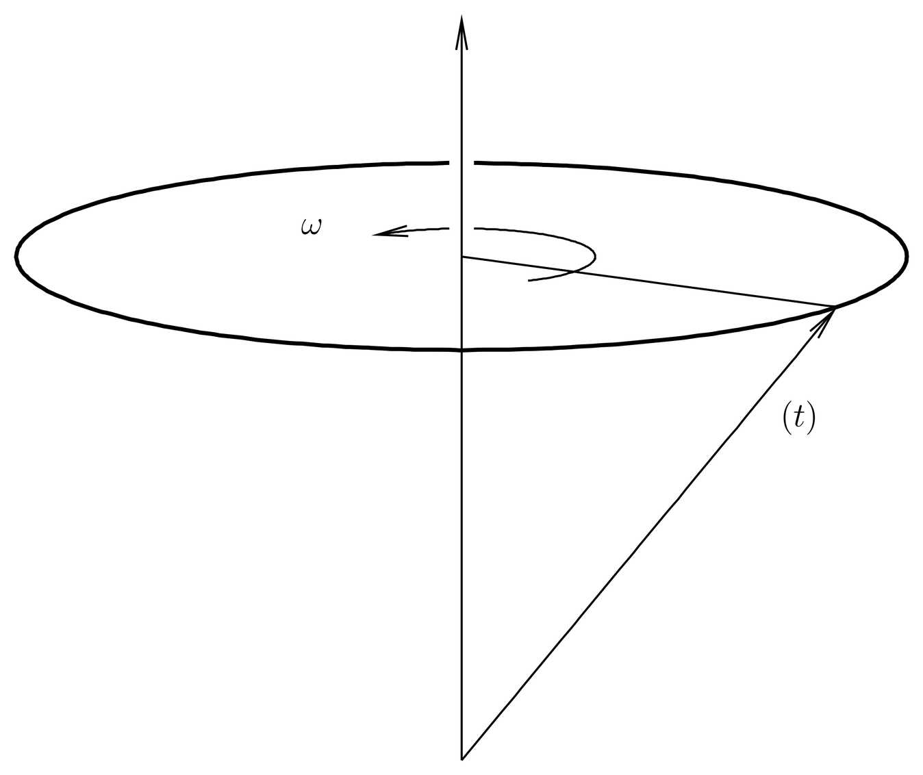
Figure 1:In a constant magnetic field, precesses about the field direction at frequency .
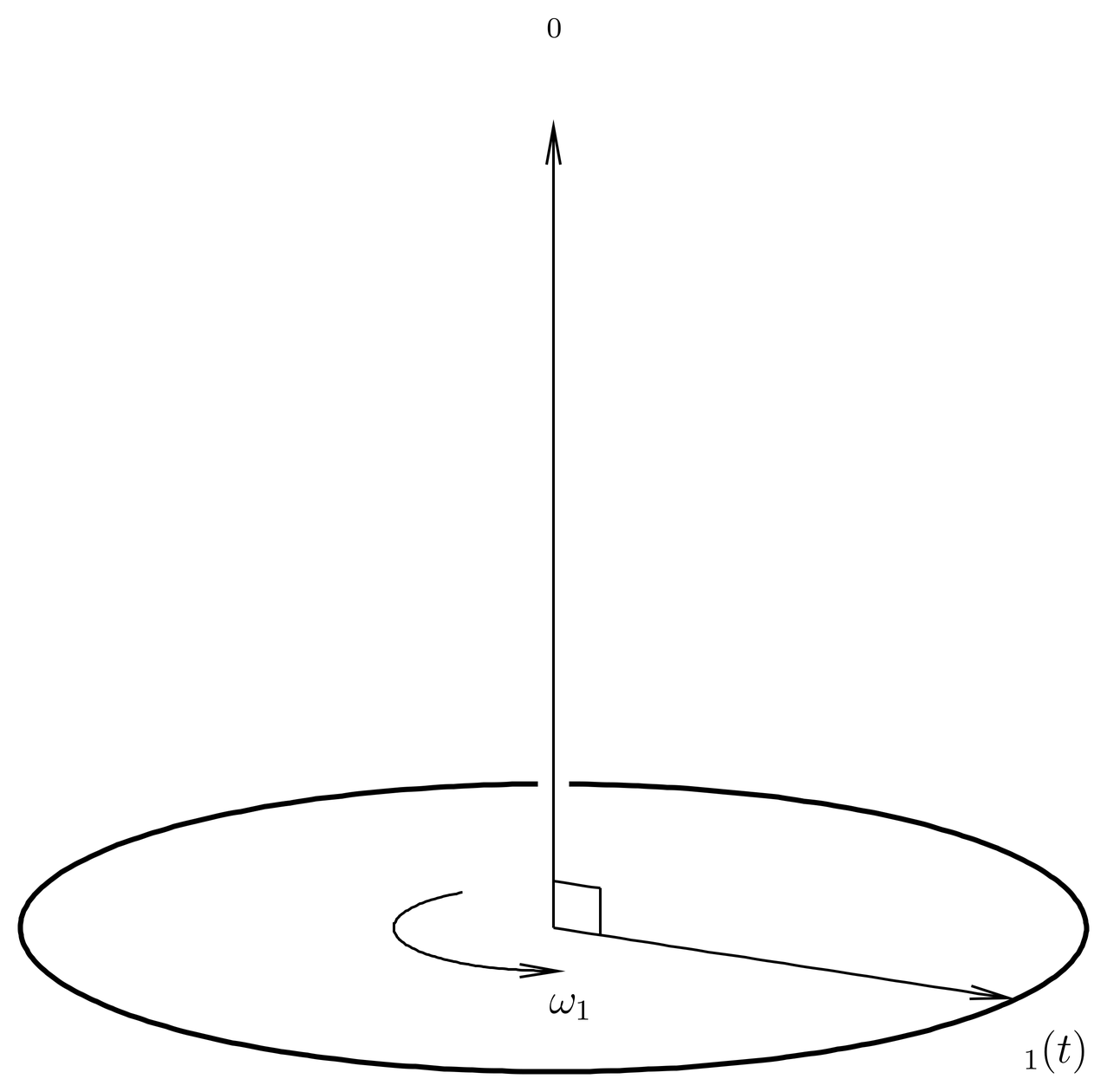
Figure 2:The field in magnetic resonance experiments consists of a constant field plus a time-dependent field that is perpendicular to and that rotates about at frequency .
Given , it is straightforward to find the time evolution of the expectation value of the spin. We have
where we have used the adjoint formula (95). We see that the expectation value of rotates counterclockwise (for ) about the direction of the magnetic field, sweeping out a cone. This is illustrated in Figure 1.
Magnetic Resonance Experiments
A more interesting case occurs in magnetic resonance experiments. Here the magnetic field consists of a constant, background field , plus a time-dependent that is perpendicular to and oscillating with some frequency . In the absence of , the spin would evolve according to a time-dependent rotation with angular velocity,
whose magnitude is
The time-dependent field is used to induce spin flips. To do this its magnitude need not be large, but its frequency should be at or near resonance with the precession frequency in the background field. Thus, the interesting case is and . Notice that is determined by the magnitude of the background field , but is the frequency of the time-dependence of , and is independent of its magnitude.
We will consider the case that rotates in a counterclockwise direction (clockwise, if ) at frequency in the plane perpendicular to , as illustrated in Figure 2. This case has the advantage that the Schr"odinger equation can be solved exactly in terms of rotation operators. We assume the magnitude of is constant, so the vector traces out a circle in the perpendicular plane. The time-dependence of can be expressed in terms of a classical rotation about the axis ,
where is a constant vector (the initial value of ) perpendicular to , and where
Another possibility for the time-dependence of will be mentioned below.
The Schr"odinger equation can now be written,
We solve this by effectively going over to a frame rotating with frequency about the axis . This cancels out the rotation of the field , giving a constant magnetic field in the rotating frame. However, as is well known, Coriolis effects in a rotating frame reproduce the effects of a magnetic field, and can be used to enhance or cancel out the effects of a true magnetic field. In the present case, in the rotating frame the effects of are partially or totally cancelled, resulting in an effective magnetic field that is the sum of a reduced magnetic field in the direction plus the constant field in the perpendicular direction.
We obtain the effect of going to a rotating frame by stripping off the time dependence
from the state vector , that is, by setting
where is a new state vector. Notice that has the same axis and angle as , defined in (49). Differentiating (52), we obtain
On the other hand, with the substitution (52) the Schr"odinger equation (50) becomes
Now we equate the right hand sides of (53) and (54) and multiply through by , to obtain
Here we have pulled the through the constant , the vectors and and the matrix , because these are just numbers or matrices and vectors composed of numbers, while , and are operators that act on kets. Now we use the adjoint formula (95), with replaced by , replaced by , and replaced by . This gives
so the dot product on the right hand side of (55) becomes
where we use (74), which expresses the invariance of the dot product under rotations. Also note that , since is the axis of . Thus (55) becomes
Rearranging this, we can write the effective Schr"odinger equation for in the form
where
or,
This is the effective magnetic field in the rotating frame. We break it up into its magnitude and direction,
so that
We also define
called the Rabi flopping frequency. Notice that if and , then (the flopping frequency is much less than the precession frequency). We will also denote the angle between and by , so that
as illustrated in Figure 3.
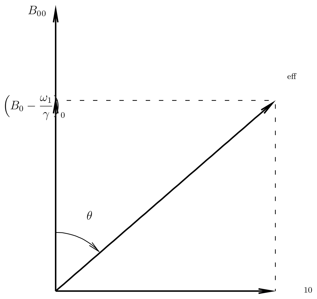
Figure 3:In the rotating frame, the field is stationary, and is reduced in magnitude by . The resulting field is , which is constant in the rotating frame.
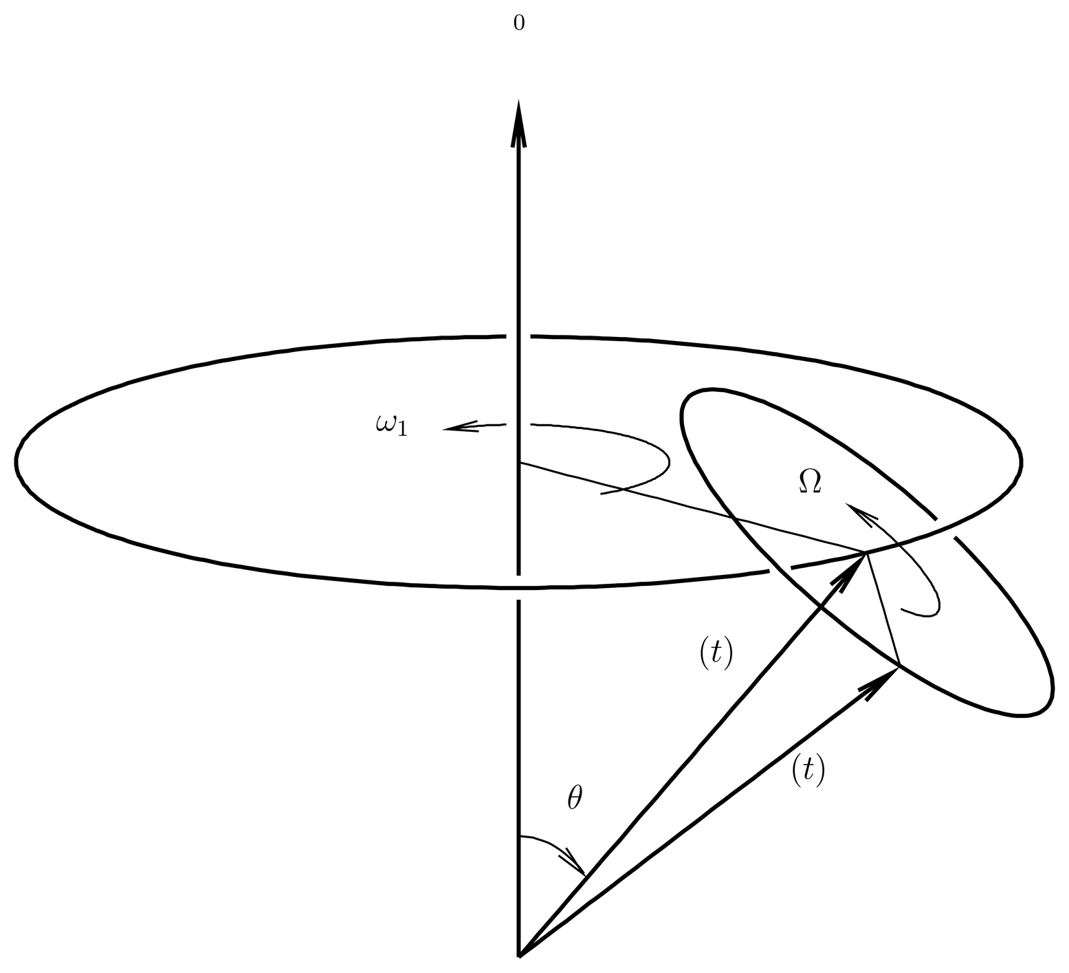
Figure 4:The expectation value of the spin precesses about the axis with frequency , while that axis itself precesses about with frequency .
The Schr"odinger equation for , (59), is the case of a spin in a constant magnetic field, so the solution is
Combining this with (52), we obtain the time evolution operator for the original Schr"odinger equation (50),
As before, we can use the solution (67) to find the evolution of the expectation value of the spin. We find,
Thus, sweeps out a cone at frequency about an axis that makes an angle with the direction , while this axis itself sweeps out a cone about at frequency . This is illustrated in Figure 4. The direction is the initial direction of the axis at , so that
(68) can be expressed explicitly in terms of the time-dependent axis by use of the exponentiated adjoint formula, (51):
which provides another way of visualizing the time evolution of .
We remark that in practice it is easier to use a different time-dependent field , given by
where we put along the -axis. This field is the sum of two counter-rotating fields,
so that if we go into the rotating frame as above then one of these fields becomes constant while the other is rotating in the opposite direction at a frequency . This is much higher than under the conditions we have posited, so the oppositely rotating field causes only small changes in the solution we have given. High frequency perturbations generally have only a small effect on a system because before the effect has a chance to build up, the perturbation changes sign and starts working in the opposite direction.
A Sample Calculation
Suppose we have a spin- particle, initially in an up state, , and suppose we ask for the probability at a later time of finding the spin in the down state . We take the direction to lie along the -axis, and we place the vectors and in the - plane. To compute the probability amplitude for the transition, we use (67) to obtain
But since
we have
Thus, the transition probability is
In the resonant case, , we have and , so that the axis of the rotating cone lies in the - plane. In this case, the transition probability (77) reaches a maximum value of unity when .
Problems
Problem 1.
Consider a particle of spin 1 and magnetic moment in the magnetic field,
employed in magnetic resonance experiments (assume ). If at , the particle is in state , find the transition probabilities as a function of time.
Problem 2.
As noted in Sec.~\secr\cn.6, the evolution of a spin in a magnetic field, with an arbitrary time dependence, is a rotation. That is, we can write
where is a rotation operator that depends on Euler angles , and where the Euler angles are functions of time. Therefore the Schr"odinger equation for must imply equations of evolution for the Euler angles.
Let be defined by
Find equations of motion for the Euler angles, assuming is given. Your answer will be identical to the equations of motion of the Euler angles in classical rigid body theory (for given ).
Problem 3.
In this problem we look at some numbers that are relevant in practice for magnetic resonance on protons. Protons are the usual nucleus of interest in medical imaging.
(a) A spin in a bulk sample is only partially aligned with a background magnetic field, because thermal agitation is always disrupting the alignment. The partial alignment of a spin in a magnetic field is a standard problem in statistical mechanics. The alignment can be increased by going to lower temperatures, but this is obviously not feasible in medical imaging.
Consider a biological sample at 300K in a magnetic field of 6T (for example, you in an MRI device). After a certain relaxation time, the nuclear spins will reach thermal equilibrium with their environment (a heat bath). Calculate the fractional magnetization of protons under such circumstances (the magnetization compared to the maximum we would have at 0K). Finally, for a sample of water under the conditions indicated, compute the magnetization due to protons in Gauss. The magnetization is the magnetic dipole moment per unit volume.
(b) Compute the spin precession frequency of protons in a field of 6T. Express your answer in Hz.
(c) An RF electromagnetic wave is used to create the rotating magnetic field [see (48).] If the power flux of the wave is , what is the Rabi flopping frequency when the wave is in resonance with the precession? Express your answer in Hertz. Remember that we do not want to cook the patient.
Problem 4.
In this problem we seek to understand the circumstances under which the magnetic moment is proportional to the angular momentum, working with a classical model. The case of a single charged particle in a circular orbit was covered in the notes (see Eq.~(\eqr\cn.11)).
Consider a system of classical charged particles of masses and charges , . Let the positions and velocities of the particles be and . We assume the classical Hamiltonian is invariant under rotations, so the total classical angular momentum,
is conserved. The current produced by particle at position is
Compute the magnetic moment according to (1) and show that if all the particles are identical, then and are proportional. What is the constant of proportionality?
This calculation applies to a classical model of an atom with an infinitely heavy nucleus because all the electrons have the same mass and charge. The nucleus does not have the same mass and charge as the electrons, but in the limit that its mass is infinite its velocity is zero so it does not contribute to either the angular momentum or the magnetic moment and the result still holds.
A similar calculation in quantum mechanics shows that the orbital contribution to the magnetic moment of atoms, including multielectron atoms, is proportional to the orbital angular momentum with the same proportionality factor as in the classical calculation, that is, with a -factor of 1.
This calculation does not apply to a classical model of a compound nucleus, because the protons and neutrons do not have the same charge (and, to a lesser extent, because their masses are not exactly equal). In any case, in both atoms and nuclei, we must take into account the spins of the particles, as well as the orbital angular momentum, in a realistic, quantum mechanical accounting of the magnetic moment.
In general, the classical magnetic momennt is not proportional to the angular momentum; and the quantum mechanical magnetic moment operator is not proportional to the quantum mechanical angular momentum operator. This applies to the orbital contribution, the spin contribution, and to the total. Nevertheless, it turns out that in weak magnetic fields, the effective quantum mechanical magnetic moment and the total angular momentum are proportional, with some effective -factor, on the energy eigenspaces of typical quantum systems. This fact will be explained in The Weak Field Zeeman Effect.