13. Representations of the Angular Momentum Operators and Rotations
Introduction
In 12. Rotations in Quantum Mechanics, and Rotations of Spin-1/2 Systems\ we introduced the concept of rotation operators acting on the Hilbert space of some quantum mechanical system, and set down postulates [(2)--(4)] that those operators should satisfy. From these we defined the angular momentum operators [in (11)] and showed that the multiplication law for rotations implies that the components of satisfy the commutation relations (24). Finally, we examined the case of spin- systems, for which , finding a double-valued representation of the classical rotations by unitary operators, or, better, a single-valued representation of spin rotations by the classical rotations, .
In these notes we generalize the treatment of rotations of spin- systems, which was presented in 12. Rotations in Quantum Mechanics, and Rotations of Spin-1/2 Systems, to an arbitrary quantum mechanical system. We assume that rotation operators are defined on the Hilbert space of our system. In practice this includes almost any system one can think of. The generators of the rotations are the components of the angular momentum , a vector of Hermitian operators that satisfy the commutation relations
In terms of these, the rotation operators in axis-angle form are given by
Conversely, the angular momentum operators are given in terms of the rotation operators by
where in comparison to (2) we have set . Knowledge of the rotation operators implies knowledge of the angular momentum, and vice versa.
In general, symmetries impose a geometrical structure on the Hilbert space of a quantum system. That is, they cause the Hilbert space to be broken up into a family of orthogonal subspaces, each of which contains states that transform in a certain way under the symmetry operations. For example, parity in one-dimensional wave mechanics causes the Hilbert space of wave functions to decompose into two orthogonal subspaces, containing the wave functions that are even or odd under parity. By defining a set of orthonormal basis vectors in each of the subspaces of a certain symmetry class we obtain a so-called symmetry adapted basis that is especially convenient for studying the symmetry properties of the system and for numerical work. If the Hamiltonian commutes with the symmetry in question, then it is possible to choose a symmetry adapted basis that is also an energy eigenbasis, and these are especially convenient for studying the system.
We will see that rotations and the associated the angular momentum operators can be used to construct a symmetry-adapted basis on the Hilbert space, what we will call a standard angular momentum basis. This basis will lead to a decomposition of our Hilbert space into an orthogonal set of invariant, irreducible subspaces, the vectors of which transform in an especially simple manner under rotations.
Although we will speak in these notes of a Hilbert space which is the ket space or state space of a quantum mechanical system, and we will use the Dirac notation for the (ket) vectors of this space, there are a wide variety of other vector spaces to which the same analysis applies. These include other types of ket spaces, such as subspaces of a given ket space, or tensor products of ket spaces. They also include spaces that are not ket spaces at all, such as vector spaces of operators (which we will take up in 20. The Wigner-Eckart Theorem), or ordinary, three-dimensional, physical space (certainly a space upon which rotations act), or spaces of classical fields (for example, electric and magnetic), in which the standard angular momentum basis is related to the multipole expansion of those fields. Thus, the treatment of this set of notes is actually quite general.
The spectrum of and 
We will now explore the consequences of the angular momentum commutation relations (1) for the spectrum of various angular momentum operators. It is rather amazing how much follows from the commutation relations alone. We use a variation of Dirac’s algebraic method that was applied in Dirac’s Algebraic Method for the Eigenvalues to the harmonic oscillator.
We begin by constructing the nonnegative definite operator ,
which, as an easy calculation shows, commutes with all three components of ,
Since commutes with , it commutes also with any function of . Let be such a function, for example, could be , , , , , or the rotation operators . Then
An operator such as that commutes with all the generators of a group is called a Casimir operator.
Since and commute, we can construct simultaneous eigenkets of and any one of the components of . However, since these components do not commute with each other, we cannot find simultaneous eigenbasis of more than one component of . By convention we choose the 3-component, and look for simultaneous eigenkets of and .
We denote the eigenvalues of and by and , respectively, so that and are dimensionless. We note that and must be real, since and are Hermitian, and that , since is nonnegative definite.
We will begin by assuming for simplicity that the operators form a complete set of commuting operators by themselves, so that their simultaneous eigenstates are nondegenerate and form a basis in the Hilbert space. Later we will return to what happens when this is not so.
The eigenvalue equations determine the kets to within a normalization and a phase. We assume the kets are normalized, so that the set forms an orthonormal basis in the Hilbert space,
We assume that some arbitrary (at this point) phase conventions have been chosen for the kets . The eigenvalue-eigenket equations are
We will be interested in the simultaneous eigenvalues , which can be represented as “eigenpoints” in the - plane. At this point all we know is that , so the eigenpoints must lie in the upper half plane.
To find these eigenvalues we introduce the ladder or raising and lowering operators,
These are Hermitian conjugates of each other,
and they satisfy the commutation relations,
as well as the relations,
The operators and are nonnegative definite.
Let us take some normalized eigenket of and , for some as yet unknown values of and , and sandwich it around (13) and (14). We find
where the inequalities follow from the fact that the left hand sides are the squares of ket vectors [see (28)]. Taken together, these imply
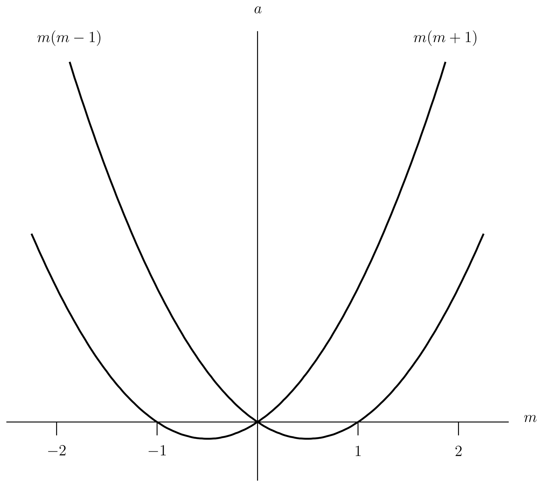
Figure 1:Functions and .
![Function \max[m(m+1),m(m-1)], with maximum and minimum values of m for a given value of a. We define j=m_max, which makes j a function of a and vice versa, that is, a=j(j+1).](/Quantum-Mechanics/build/repsamos-fig02-b15793ffcfe1c3c91af9a594af619710.png)
Figure 2:Function , with maximum and minimum values of for a given value of . We define , which makes a function of and vice versa, that is, .
The functions are plotted in Figure 1, and the maximum of these two functions is plotted in Figure 2. The maximum function is symmetric about , and everywhere. According to (17), the eigenpoints must lie in the shaded region in Figure 2 or on its boundary.
Let be an eigenvalue of . A value of is indicated by a horizontal line in Figure 2, which intersects the boundary of the shaded region in two points. There must be one or more eigenpoints on this line, whose values lie between certain maximum and minimum values, which are functions of . Let us define
so that
as shown in Figure 2. The coordinates of the two interpoints are on the left and on the right, so is a function of given by
with . Then we have
It turns out to be more convenient to parameterize the eigenvalues and eigenkets of by instead of , so henceforth let us write for the eigenvalue of instead of , and let us write instead of for the eigenkets of and . Then (8) become
and the orthonormality conditions (7) become
We also rewrite (15) and (16) with this change of notation, noting that the right hand sides can be factored,
Also let us replace the - plane with the - plane, so that Figure 2 becomes Figure 3.
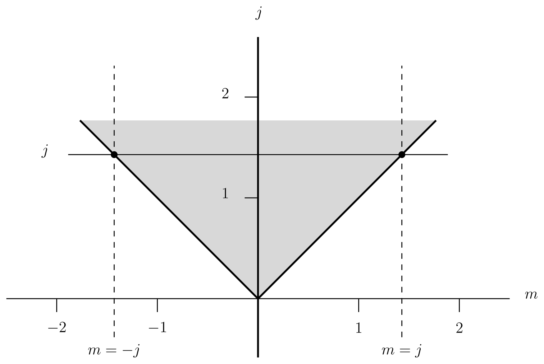
Figure 3:ure Figure 2 redrawn with as the vertical coordinate instead of , where . The bounding lines are now , and for a given value of (the horizontal line) is bounded by .
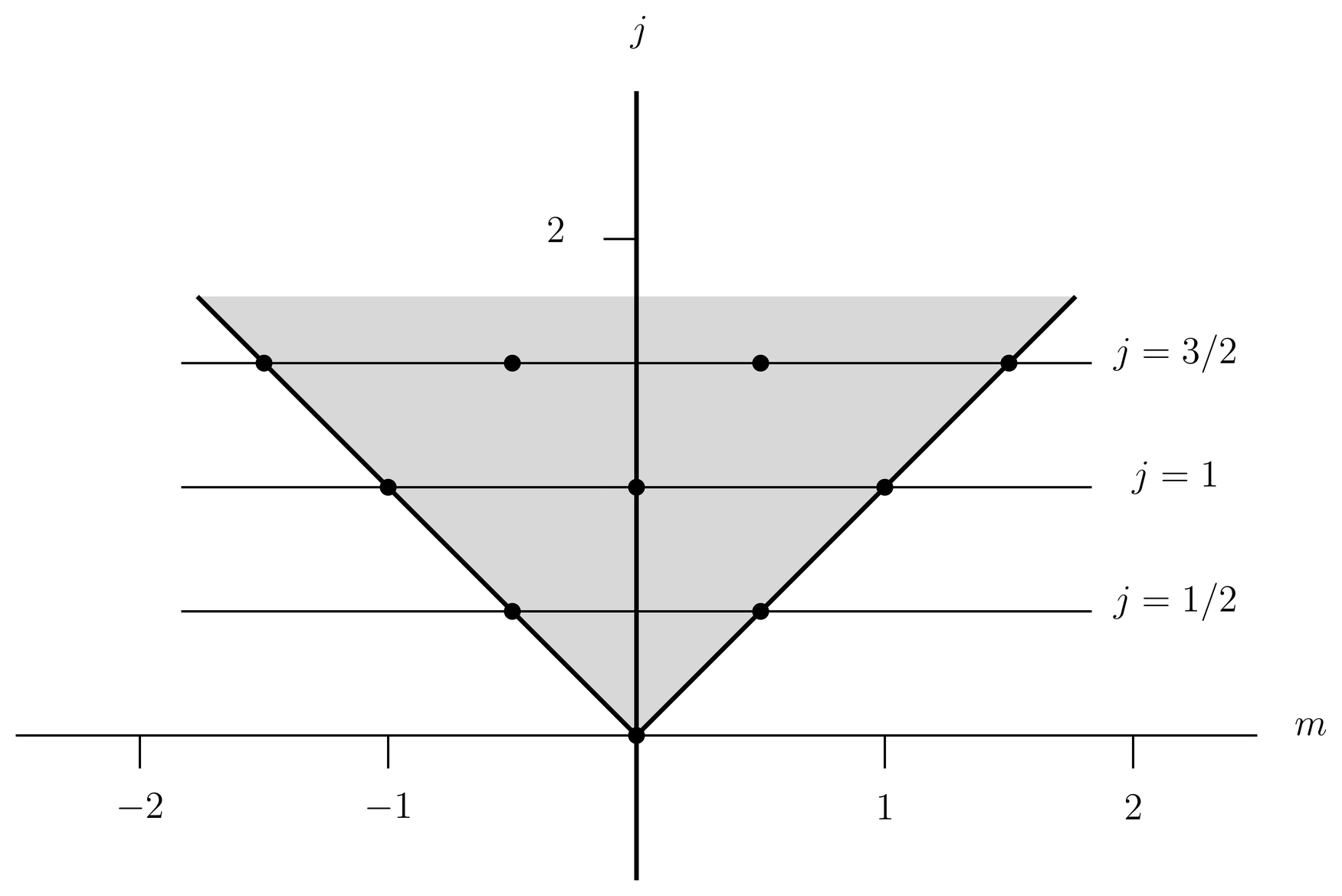
Figure 4:Spots are shown in - plane for allowed eigenvalues. Whether a given value (a horizontal line in the figure) actually occurs depends on the application; but if it does occur, then all -values (the spots along the horizontal line, between and , in integer steps) occur.
The behavior of as a raising operator is indicated by the following theorem.
In this theorem, we assume that is an eigenket of and with the indicated quantum numbers, and that it is normalized as indicated by (23), and, in particular, that . We have to worry about the possibility that is zero, because zero vectors are not usually considered eigenvectors of anything. The theorem says that does not change the quantum number but it raises by one unit. The theorem is easily proved with the help of the commutation relations (11) and (12),
Similarly, we can show that if the state does not vanish, then it is an eigenket of and with eigenvalues and , respectively. That is, does not change the quantum number but it lowers by one unit.
We must worry about the case . Since a vector vanishes if and only if its square vanishes, we have if and only if
where we use (24). But this holds if and only if either or . But is impossible in view of (21), so we see that
Similarly, we find that
From this it immediately follows that
where is an integer, for if this were not so, we could successively apply to (which is nonzero), and generate nonzero kets with successively higher values of until the rule (21) was violated. Similarly, we show that
where is another integer. But taken together, (31) and (32) imply , that is, is a nonnegative integer. Thus, the only values of allowed by the commutation relations (1) are nonnegative integers or half-integers,
When we say that belongs to the indicated set of values (integers and half-integers), we mean that the commutation relations alone tell us that can take on only these values. They do not tell us which of these values actually occur in a specific application.
For example, speaking of the spin of a spin- particle, (that is, the spin) takes on only the value . But in a central force problem, in which the energy eigenfunctions are and is identified with the orbital angular momentum , (that is, ) takes on all possible integer values but none of the half-integer values.
But in any application, if some value does occur, then all values in the range,
also occur, for if any one value in this list occurs, that is, if a nonzero eigenket exists, then all other nonzero eigenkets with the same value but other values in the range (34) can be generated from the given one by raising and lowering operators. Thus, the eigenvalue of is -fold degenerate. The allowed eigenvalues of and are illustrated as spots in the - plane in Figure 4.
Superselection Rules
The commutation relations (1) alone only tell us that the values that occur in any application belong to the set (33), consisting of nonnegative integers and half-integers. It turns out, however, that in physical applications the values of that occur are either all integers or all half-integers. In nonrelativistic quantum mechanics, this is is because the spins of particles are either integers or half-integers, and orbital angular momenta are always integers. That is, if is the Hilbert space of a physical system and if rotation operators (and therefore angular momentum operators) are defined on it, then the eigenvalues of that occur in are given either by integer or half-integer , never a mixture of the two. This is sometimes stated by saying that there is no physical meaning to linear combinations of states with integer and half-integer . This type of restriction is called a “superselection rule.”
This superselection rule only applies when the rotations in question represent physical rotations in 3-dimensional space, as discussed in 11. Rotations in 3-Dimensional Space. Sometimes there arise operators of the same mathematical form as physical rotations but without this physical meaning, for example, in the two-dimensional, isotropic harmonic oscillator that forms the basis of Schwinger’s treatment of angular momentum theory (see Prob. Paragraph). In such cases linear combinations of integer and half-integer can and do occur.
Phase Conventions and Matrix Elements of 
Since by assumption the simultaneous eigenkets of and are nondegenerate, the state must be proportional to ,
where is a complex number. Squaring both sides and using (25) we obtain
or,
where is a phase. Let us write out these equations starting with the “stretched state” and lowering in unit steps,
etc. These show that if we choose the phase of the stretched state arbitrarily, then we can absorb the phases into the phase conventions for the states for , thereby linking the phase conventions of all the states for fixed to that of the stretched state . This gets rid of the phase factors, and gives
Similarly, must be proportional to ,
where is a complex number. Applying to both sides, on the left we obtain
where we use (13), whereas on the right we obtain
where we use (39). This allows us to solve for , and altogether we obtain
These phase conventions cause the matrix elements of in the basis to be real and positive. These phase conventions are standard and convenient in the theory of angular momentum and rotations, but there is no physics in them.
With these phase conventions we can use a little induction to express an arbitrary basis vector as a lowered version of the stretched state ,
This may be compared to (40) for the harmonic oscillator. The basis that we have constructed is what we shall call the standard angular momentum basis for the Hilbert space in the case we are considering (where eigenkets of and are nondegenerate).
Matrices in the Standard Angular Momentum Basis
For practical calculations we often require the matrix elements of functions of the angular momentum in the standard angular momentum basis. Because of the commutator (6), all these matrices are diagonal in the quantum number . That is, we have
so either or . Thus we can write
in which the values on the two sides of the last matrix element are the same. As we say, functions of the angular momentum do not mix together subspaces with different values of . As a result, the matrices of any operator in the standard angular momentum basis are specified by a set of submatrices, one for each value, whose rows and columns are indexed by and and whose size is .
We can easily give explicit formulas for some of these matrices. The matrices of are especially simple, since the standard angular momentum basis is an eigenbasis of ,
The matrix of for a given value of is a multiple of the identity. Similarly, the standard angular momentum basis is also an eigenbasis of , so
The matrix of for a given value of is diagonal, but it is not a multiple of the identity.
The matrices of and can be obtained from (39) and (43) by multiplying on the left by and using the orthonormality of the basis. This gives
where we have swapped and in the results. Notice that the matrix for is the transpose of that for , since and for real matrices the Hermitian conjugate is the same as the transpose. Also, since and can be expressed in terms of ,
it is easy to write down the matrices for and . Note that since the matrices of are real, by (51) those of are real and those of are purely imaginary.
Thus we know the matrix elements of all three components of in the standard angular momentum basis. From these one can find the matrix elements of any function of , such as the rotation operators . Notice that all these matrices are diagonal in (the matrix elements are proportional to ), so the matrix elements themselves depend only on , and .
Let us look at some specific examples. For a given operator we present the matrix with components , with labeling the rows and labeling the columns, and with magnetic quantum numbers starting with the stretched value and proceeding down to in integer steps as we move across rows or down columns.
In the case the matrices for and are
We do not display the matrix for since it is just the transpose of the matrix for . But from and we compute the matrices for and ,
We see that when , , the same conclusion we reached in 12. Rotations in Quantum Mechanics, and Rotations of Spin-1/2 Systems{} (and note that we are confusing an operator with the matrix representing that operator in the standard angular momentum basis).
In the case the matrices for and are
from which we obtain the matrices for and ,
In these equations we see the generalization of the Pauli matrices to the case .
In the case , the matrices for and are
We omit the matrices for and in this case, but they are easily computed.
A case not to be neglected is , for which can take on only one value, , so that all matrices are . The matrices are
The angular momentum operator is zero on a subspace in which .
Rotation Matrices
The matrices of the rotation operators are especially important, and we give them a special notation. If is a rotation operator, we define
The symbol is for German Drehung, which means, “rotation.” These matrices are also sometimes referred to as “Wigner -matrices.”
The rotation operator can be parameterized in a variety of ways, for example, in axis-angle form , in Euler angle form or as a function of a spatial rotation, . In these cases we can write , or for the corresponding rotation matrix. We can also write , to indicate the dependence of the rotation matrix on the unitary operator. Note that if is a double-valued function of , then so is the matrix .
The -matrices appear when we rotate a basis vector of the standard angular momentum basis. By inserting a resolution of the identity we have
But since the final matrix element is proportional to [see (46)], the sum reduces to just one over ,
When we apply a rotation to a basis vector , we obtain a linear combination of basis vectors with the same value of , and the -matrices give the expansion coefficients. There is no mixing of different values.
In the case the matrices for all three components of are just , so the matrix for the rotation operator is
This means that a state with is invariant under rotations, since multiplying by 1 does nothing. An example is the ground state of hydrogen, in which wave function is rotationally invariant (the angular dependence is given by , which is a constant, independent of angle). If we include the spins of the electron and proton in our description of the hydrogen atom, the ground state is still a state of (the spin singlet state, although the quantum number is usually called instead of . See 27. Hyperfine Structure in Atoms).
In the case , we have already worked out the matrices for the rotation operators in axis-angle form,
[see (27) and Prob. Paragraph(b)]. Rotation matrices in axis-angle form for higher values of can also be worked out.
The rotation matrix is especially simple in the case that , since in that case the rotation matrix, being the exponential of the diagonal matrix (48), is itself diagonal. Thus we have
This particular rotation leads to an important conclusion. When is half-integral, then so is , and we find
Thus, rotating any system of half-integer angular momentum by an angle of does not return it to its original value, but rather multiplies the state by -1. This actually applies to any axis, not just the -axis. This generalizes what we saw earlier for the special case . For all half-integer values of the representation of spatial rotations by quantum rotations is double-valued, exactly as for spin- systems. In this case the ranges on the Euler angles are modified, as seen in (61). However, in the case of integer , we have
which actually applies to any axis (not just ). For integer the quantum rotations form a single-valued representation of the spatial rotations .
Although the -matrices form a single- or double-valued representation of , depending on the value of , it can be said that they always form a single-valued representation of , the group of spin- rotations, while itself forms a double-valued representation of . Actually, it is better to say that is a single-valued representation of , which points to as the fundamental group of rotations in quantum mechanics.
Euler Angles and Reduced Rotation Matrices
In many applications the Euler angle parameterization of the rotation matrices is convenient. We write
which is the same as (58) except here generalized to arbitrary values of . By taking matrix elements and introducing resolutions of the identity we obtain
where the resolutions of the identity involve only a sum over , not over , for the same reason as in (60). But the first and third matrix elements are for rotations about the axis, which by (63) are diagonal. As for the middle rotation about the -axis, we give a special notation for it,
which we call a “reduced rotation matrix.” Altogether, we have
The reduced rotation matrix is the nontrivial part of the matrix , so only it is presented in tables of rotation matrices. Notice that since the matrices for are purely imaginary by our phase conventions, the matrices for , that is, the reduced rotation matrices, are purely real. This is a convenient aspect of the various conventions we have established, and it explains why Wigner chose the -convention for Euler angles, instead of the -convention which is common in books on classical mechanics.
We now present some examples of the reduced rotation matrices. For the case , the result is trivial:
which is a special case of (61).
For the case , we use the properties of the Pauli matrices to obtain
which is a special case of (27) (see also Prob. Paragraph).
For the case , we can find recursions among the powers of the matrix for , and sum the exponential series to obtain
For higher values of it is most convenient to use recursion relations or other methods for calculating the matrices . These matrices are tabulated in standard references on rotations in quantum mechanics. The matrix elements are closely related to the Jacobi polynomials of , and they satisfy various differential equations and recursion relations. A more elegant way of getting these matrices is to use Schwinger’s algebraic method, which converts angular momentum algebra into a version of harmonic oscillator algebra. An introduction to this subject was given in Prob. Paragraph.
Properties of the Rotation Matrices
The -matrices have many properties, of which we mention three. First, if is a rotation operator and the corresponding matrix, then the operator corresponds to the matrix . But since is unitary, so is the matrix , and we have
Next there is the representation property. If we think of the -matrices as parameterized by the unitary rotation operators , then
If we think of -matrices as parameterized by the classical rotations , then in the case of integer they form a representation of ,
In the case of half-integral they form a double valued representation of , in which each classical corresponds to two -matrices, differing by a sign. In that case we can write
with the same understandings as in (41).
Next, the transformation properties of angular momentum under time reversal, a topic that we take up in 22. Time Reversal, show that
See Prob. Paragraph.
The Grand Orthogonality Theorem
We mention one final, important property. The components of the -matrices satisfy certain orthonormality properties, when integrated over the group manifold. If we express the -matrices as functions of the Euler angles (see Secs. Euler Angles and Spinor Rotations about the Coordinate Axes), then we have
This is valid for all , both integral and half-integral. The ranges on the Euler angles given are those needed to cover , as explained in Spinor Rotations about the Coordinate Axes and by (61). These ranges are needed if is a half-integer. But if is an integer, then the second half of the range just duplicates the first half, , and (78) can be replaced by
Here the ranges on the Euler angles are those needed to cover .
A physical application of these relations occurs in the quantum theory of the rigid body. Many small molecules are approximately rigid bodies, and the theory applies to them. In the quantum rigid body the wave function can be thought of as a function on the group manifold, , whose square gives the probability density for the orientation of the molecule. In the case of the symmetric top a suitable complete set of commuting observables for the energy eigenfunctions are , where is the -component of the angular momentum with respect to the space frame and is the -component of the angular momentum with respect to the body frame. The Hamiltonian is a function of and , and the energy eigenfunctions are the components of the -matrices. The integral (79) expresses the orthonormality of these eigenfunctions.
We will not prove these orthonormality relations. Their significance is much deeper than the application to the rigid body would suggest; in fact, these are special cases of what is called the grand orthogonality theorem, which applies to the unitary repressntations of any group. Here [in (78) and (79)] the groups are and .
Degeneracies and Multiplicities
Let us now consider the general case in which the simultaneous eigenstates of and are degenerate, that is, the operators by themselves do not form a complete set of commuting operators, and their simultaneous eigenspaces are multidimensional. Let us denote the eigenspace of and with eigenvalues and by , and let us write
We wish to consider the case that .
Let us take the stretched eigenspace which has dimension , and let us choose a set of linearly independent vectors in this space. Applying to these vectors, we obtain a set of vectors that are eigenvectors of and with eigenvalues and (that is, with a lowered value of ). These vectors must lie in the eigenspace , and, as one can show, they are also linearly independent. Thus, .
Now choose a set of linearly independent vectors in and apply the raising operator to them. This creates a set of vectors that lie in the stretched eigenspace , which, as one can show, are also linearly independent. Thus, . But this is consistent with only if .
Continuing in this way, we see that all the eigenspaces for have the same dimensionality. We denote this dimensionality by , which we call the multiplicity of the given value. The multiplicity can take on any value from 0 (in which case the value does not occur) to .
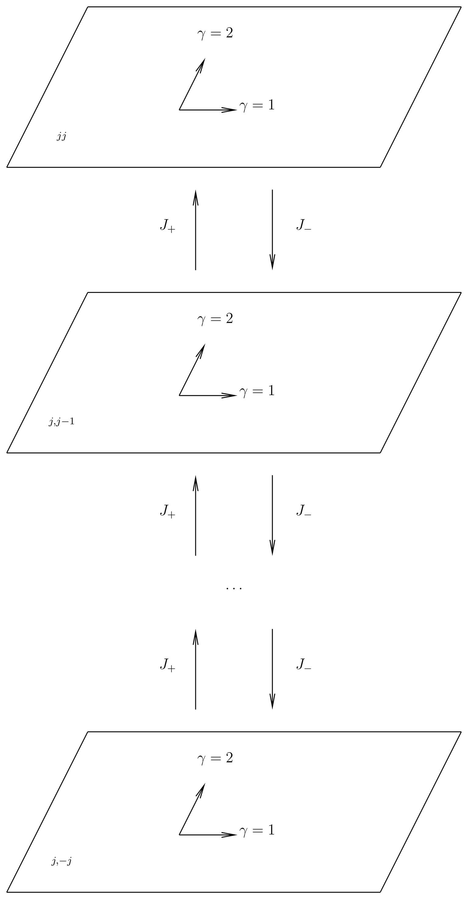
Figure 5:The standard angular momentum basis is obtained by choosing an arbitrary orthonormal basis in the stretched space , indexed by , and applying lowering operators.
Now let us choose an arbitrary, orthonormal basis in the stretched space , indexed by an index , where . See Figure 5. In practice may be the quantum number (or numbers) of one or more additional observables, that commute with both and and that form a complete set when taken with and . For example, in the hydrogen atom, a commonly used complete set of commuting observables is with quantum numbers , where takes the place of and is replaced by to indicate orbital angular momentum.
Let us call these vectors . If we apply to these, we obtain vectors in the next space down, . One can easily show that the orthogonality of these vectors is preserved under the action of . As for the normalization, it is changed by , as indicated by the square root factor in (39), but if we compensate for this we obtain an orthonormal basis in . Let us call the new vectors , that is, let us define by
Continuing in this way, we propagate an orthonormal basis from all the way down to , as in Figure 5. We call the basis vectors , and by their construction they satisfy
Equivalently, using recursion as in (44), we can write
By this construction, the raising and lowering operators change only the values, not the or values. The resulting set of vectors forms an orthonormal basis on the entire Hilbert space ,
We call the basis a standard angular momentum basis on in the general case in which by themselves do not form a complete set. It is still an eigenbasis of and ,
in which the index resolves the degeneracies.
We can now write down the matrix elements of the raising and lowering operators, as well as those of and , in the standard angular momentum basis . Multiplying (82) or (85) on the left by and using the orthonormality, we obtain
The matrix elements are diagonal in both and , and depend only on , and . Note especially that the matrix elements are independent of .
Since these properties apply to and , they apply to and as well, that is, to all three components of , and therefore to any function . For example, the matrix elements of a rotation operator in the standard angular momentum basis satisfy
where the final matrix element is just the -matrix,
Not only is this independent of , it is the same -matrix we defined in Rotation Matrices.
A practical way of thinking about these conclusions is to say that in standard angular momentum basis , the extra index just goes along for the ride insofar as angular momentum or rotation operators are concerned.
Invariant, Irreducible Subspaces
In (59) and (60) above we considered the action of a rotation operator on a vector of the standard angular momentum basis. Let us reconsider that action now that we have the extra index in the basis. By inserting a resolution of the identity, we have
where is a rotation operator, where the and sums can be done because of the Kronecker deltas in (89) and where we have used (90). The rotation operator mixes neither spaces of different nor spaces of different . The same conclusion applies to any function of the angular momentum.
We see that if we rotate a basis vector we get a linear combination of vectors with the same and but different . This calls attention to the subspaces,
which are invariant under the action of any function of the angular momentum , notably the rotation operators. That is, if we take any vector in one of these subspaces and apply any angular momentum or rotation operator to it, we obtain another vector in the same subspace. Note that
The concept of a subspace that is invariant under the action of an operator was touched upon previously in Simultaneous Eigenbases of Commuting Observables. Note that the subspaces are orthogonal to one another, that is, every vector in one such space is orthogonal to every vector in any other such space.
The subspaces are not only invariant under the action of the rotations, they are also irreducible. This means that they contain no smaller subspaces that are invariant under the rotations. These invariant, irreducible subspaces play an important role in any system upon which rotations act, and we shall refer to them frequently. We will call them irreducible subspaces for short. You may think of them as spaces spanned by vectors connected by raising and lowering operators. The entire Hilbert space upon which rotations act is decomposed by the action of the rotations into a direct sum of mutually orthogonal, invariant, irreducible subspaces,
This is a basic geometrical structure imposed on the Hilbert space by the action of rotations.
An important application of these concepts occurs in any system that is isolated from its environment, so that its energy does not depend on its orientation. Such systems are very common in applications. In this case the Hamiltonian commutes with all rotation operators, which, it turns out, implies that each energy eigenspaces consists of one or more irreducible subspaces, usually just one. In the usual case that an energy eigenspace consists of a single irreducible subspace, the energy level is characterized by an angular momentum quantum number and is -fold degenerate. We will explore these facts in greater detail in 20. The Wigner-Eckart Theorem.
The concept of an invariant, irreducible subspace plays an important role in the representation theory of any group. We have developed the idea here in an ad hoc manner, suitable for the rotation group and the applications we will consider.
Generalized Adjoint Formula
We recall that we derived a version of the adjoint formula for classical rotations in (48), and later we found an analogous formula, (35), for spin- rotations. We now generalize this to arbitrary representations of the rotation operators. The generalization is obvious; it is
where and . Notice that the left hand side is quadratic in , so in the case of double-valued representations of , it does not matter which operator we choose to represent the rotation .
To prove (95), we define the operator vector,
and we note the initial condition,
Next we obtain a differential equation for :
The solution is
which is equivalent to the adjoint formula (95).
Finally, we can dot both sides of (95) by and exponentiate, to obtain a formula analogous to (51). After placing 0 subscripts on and for clarity, the result is
where and are corresponding quantum and classical rotations. This is an exponentiated version of the adjoint formula, similar to Eq.~((51). Notice again that the left hand side is quadratic in , so that in the case of double-valued representations it does not matter which operator we choose to represent the rotation . (101) is an exponentiated version of the adjoint formula (95).
Problems
Problem 1.
A molecule is approximately a rigid body. Consider a molecule such as , , or , which is not a diatomic. First let us talk classical mechanics. Then the kinetic energy of a rigid body is
where is the angular momentum vector with respect to the body frame, and are the principal moments of inertia. The body frame is assumed to be the principal axis frame in (102). The angular velocity of the rigid body is related to the angular momentum by
where is the moment of inertia tensor. When (103) is written in the principal axis frame, it becomes
Finally, the equations of motion for the angular velocity or angular momentum in the body frame are the Euler equations,
By using (104) to eliminate either or , (105) can be regarded as an equation for either or . The Euler equations are trivial for a spherical top (), they are easily solvable in terms of trigonometric functions for a symmetric top (), and they are solvable in terms of elliptic functions for an asymmetric top (, , all unequal). The symmetric top is studied in all undergraduate courses in classical mechanics.
(a) In quantum mechanics, it turns out that the Hamiltonian operator for a rigid body has exactly the form (102). The angular momentum satisfies the commutation relations,
with a minus sign relative to the familiar commutation relations because the components of are (in this problem) measured relative to the body frame. (We will not justify this. If the components of were measured with respect to the space or inertial frame, then there would be the usual plus sign in (106).) Compute the Heisenberg equations of motion for , and compare them with the classical Euler equations. You may take (103) or (104) over into quantum mechanics, in order to define an operator to make the Heisenberg equations look more like the classical Euler equations. (Just get the equation for , then cycle indices to get the others.) Make your answer look like (105) as much as possible.
(b) It is traditional in the theory of molecules to let the quantum number of (referred to the body frame) be . Write the rotational energy levels of a symmetric top () in terms of a suitable set of quantum numbers. Indicate any degeneracies. How is the oblate case () qualitatively different from the prolate case ()? Hint: In order to deal with standard commutation relations, you may wish to write , so that .
Problem 2..
A spin-1 particle has the component of its spin in the direction
measured, and the result is . Subsequently is measured, with various probabilities of the three possible outcomes.
Let be a rotation that maps the axis into , that is, let
Express the aforementioned probabilities in terms of the matrix, . Work out this matrix to find the probabilities explicitly. You may use tables of -matrices.
Problem 3..
The adjoint formula (\eqr\cn.91) is important in applications. The proof above uses a differential equation in the angle . The following is a more pictorial approach. It is based on the idea that finite rotations can be built up as the product of a large number of small rotations.
First show that if (95) is true for two rotation operators and , and the corresponding classical rotations and , then it is true for the products and . Then show that (95) is true for infinitesimal rotations. This is sufficient to prove the formula.