36. Introduction to Time-Independent Scattering Theory and Scattering from Central Force Potentials
Introduction
In 34. Time-Dependent Perturbation Theory{} we considered some scattering problems as an application of time-dependent perturbation theory, taking a time-dependent approach. In these notes we take a time-independent approach to potential scattering in three dimensions, that is, we will be interested in energy eigenfunctions of the Schr"odinger equation,
for positive energies . These solutions must satisfy certain boundary conditions to be useful in scattering theory. These energy eigenfunctions are part of the continuous spectrum so they extend to infinity and are not normalizable. Thus, they do not represent the state of physical particles, although they can be thought of as a limit of such states.
For the sake of generality we do not at first assume that the potential is rotationally invariant, but as usual in scattering theory we assume that it approaches zero with distance,
where . In fact, the simplest case is the one in which faster than as (see Asymptotic Form of the Radial Wave Functions). This excludes the case of the Coulomb potential or potentials with a Coulomb tail, which are important in practice but which require special techniques.
We will speak of the scattering of a particle by the potential , as if it were a fixed potential in space, but in reality the beam particle interacts with a target, which often is another particle. Then a proper treatment requires us to take into account the dynamics of both particles. The changes necessary to do this were discussed in some detail in 34. Time-Dependent Perturbation Theory. For now we simply note that if the target is very massive, then it can be thought of as producing a potential for the beam particle that is fixed in space (that is, in an inertial frame), as we shall assume in these notes.
We begin by examining the boundary conditions that the desired solutions of the Schr"odinger equation should satisfy in a scattering problem, in order to develop an intuitive picture of what they look like. This leads to a definition of the scattering amplitude and its relation to the differential cross . We then specialize to the case of central force potentials, for which the Schr"odinger equation is separable in spherical coordinates and for which many special results are available. We devote some attention to hard sphere scattering, which is probably the most tractable central force scattering problem, and which illustrates many features of scattering from more general potentials. Finally we discuss the optical theorem in the context of potential scattering in three dimensions, an exact result that has many generalizations.
Classical Scattering: The Steady State
We begin by considering a classical model of a scattering experiment. A beam of particles is directed at a target, as illustrated in Figure 1. We imagine that all the particles have the same momentum , and that the density of particles is uniform across the beam. In reality the beam has to be turned on at some time, so we can imagine a time-dependent problem in which the beam particles first approach the scatterer, then begin to interact with it, and then produce an outward traveling front of scattered particles. If we stand at any given point and wait, then initially there are no scattered particles, then the front arrives and we start to see them, and after the front has passed we reach a steady state, in which the flux of scattered particles is constant in time. The farther we are from the scatterer, the longer we have to wait for a steady state to be achieved, but eventually it will happen.
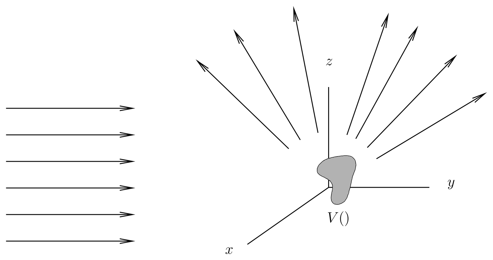
Figure 1:Classical scattering. A beam of particles, all with the same momentum , is directed against a target.
To obtain an idealized steady state we can imagine that the time at which the beam is switched on recedes to , while the source of the beam also recedes to infinity, so that we have a steady beam coming in from infinite distance in the upstream direction. We can further idealize the situation by letting the final time advance to , so that a steady flux of scattered particles exists at all spatial locations.
In this steady state, at any spatial point we have a definite flux of scattered particles, and, if we are inside the beam, also a flux of incident particles. If we are at a distance from the scatterer large enough that the potential can be neglected, then the kinetic energy of the scattered particles is the same as that of the incident particles, because the scattering is elastic. That is, when a particle gains kinetic energy by falling into the potential well, it loses the same amount when climbing back out again (or if the potential is positive it will lose kinetic energy on entering the potential, and then gain it back when exiting).
There is also the question of how wide the beam is. Real beams have a finite width, which we normally make much larger than the range of the potential (however that is defined). It is worth noting that in classical scattering the total cross is nominally infinite, unless the potential rigorously vanishes outside some radius. That is because if goes to zero only gradually as , then there is some small angle of scattering, even at large impact parameters. Most of the infinite cross that results in such a case is due to small angle scattering, so diverges as . Most of this small angle scattering might well be of no practical interest, but to see it one would need a beam that is infinitely wide (another idealization). In quantum mechanics, as we will see, total cross s are finite if the potential dies off rapidly enough with distance (it need not rigorously vanish beyond a certain radius).
Notice that if we extend the width of the beam to infinity, then (with the other idealizations we have made) the classical stationary state is uniquely determined by the momentum of the incident beam, that is, the momentum it has far upstream at a large distance from the scatterer.
The Stationary State in Quantum Scattering
In quantum mechanics a stationary state is usually defined as an energy eigenstate, which with the time-dependence has a wave function of the form . The wave function is not stationary, but the probability density and current are. Thus it is plausible that the stationary state we have just described in classical scattering should correspond to an energy eigenstate in quantum scattering.
It is not hard to visualize such an eigenfunction but there are several idealizations that must be understood. For example, as in the classical case, the steady state can be realized as the limit of a time-dependent situation. We proceed intuitively. Probably the simplest way to realize this limit is to let the initial state be a wave packet, for example, a Gaussian wave packet, whose expectation value of momentum is and whose spread in momentum is some . We will be interested in the limit so that the initial state has a well defined momentum in the limit. But the width of the wave packet in real space is , which goes to as . As it does so, the value of the normalized wave function goes to zero, since the wave function is spread over larger and larger regions of space. Therefore it is convenient to deal with unnormalized wave functions, and to require that the magnitude of at the center of the wave packet remain finite as . This means that in the limit the wave function has an infinite norm. As this limit is approached, the middle of the wave packet looks more and more like a plane wave with momentum .
We wish the wave packet at the initial time to lie far enough upstream that is has essentially no interaction with the potential. The wave packet is aimed at the target, but it evolves according to the free particle Hamiltonian until the leading edge reaches the region where the potential is effective. This guarantees that the initial wave packet does not have any components along the bound states of the potential , since any such bound state wave functions are localized in the neighborhood of the potential. We do not want such components in the initial wave packet, since the bound states are not scattering states; bound states evolve in time simply by oscillating in place, without scattering. However, since the size of the wave packet goes to in the limit , we must pull the center of the initial wave packet farther and farther away from the scatterer to guarantee that it has no overlap with the potential at the initial time. Then we must wait for a longer and longer time for the wave packet to reach the scatterer.
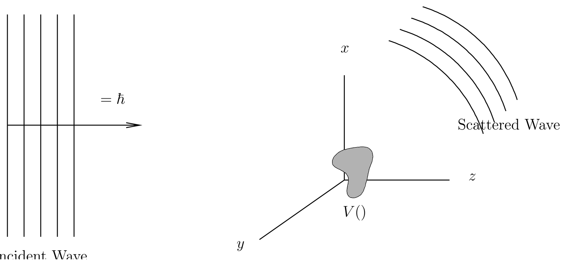
Figure 2:Quantum scattering by a potential . Incident and scattered waves are shown.
Thus there are several interlocking limits that must be taken at once, but when is small and we wait until the center of the wave packet has reached the scatterer, then for some time around this time and for some distance away from the scatterer we have a nearly steady state, in which a wave that locally looks like a plane wave is incident on the scatterer, and a scattered wave is radiating outward from the scatterer. In the limit we achieve a quantum steady state that is illustrated in Figure 2 and that resembles the classical steady state described in Classical Scattering: The Steady State. The quantum steady state that results in the limit depends only on the initial momentum .
Boundary Conditions
If we are far from the scatterer then in the resulting steady state we see two waves, an incident wave which is a plane wave of momentum and a scattered wave, radiating away from the scatterer. To rigorously define the decomposition of the total wave into an incident wave and scattered wave which is valid everywhere (even where the potential is active), we write the exact solution to the Schr"odinger equation as
where the indicent wave is a plane wave of momentum ,
and where is defined as the difference between the exact and incident wave, so that (3) is true. Also, in the asymptotic region, at large where the potential is negligible, we require that the scattered wave consist of purely outgoing waves, moving in the radial direction away from the scatterer.
If we conceive of the potential has having some well defined range then the angle subtended by the scatterer is nonzero at any finite radius , so the “outward” direction is not precisely defined. This is especially clear in the case that the potential is not rotationally invariant, so that it has no well defined center. But as the angle subtended goes to zero, and the radial direction does become well defined. In this limit, we require that the scattered wave have the form
where the symbol means that we are giving the asymptotic form of the scattered wave, valid when . More precisely, this symbol means that the left hand side equals the right hand side, plus corrections that go to zero more rapidly as than does the right hand side. For example, there may be corrections of order that are not shown. The asymptotic form in (5) indicates a wave that is traveling outward in the radial direction (as we see if we attach the time-dependent factor ), and which has an angular dependence given by the function .
In the asymptotic region both the incident wave and the scattered wave must satisfy the free particle Schr"odinger equation, assuming the potential in (1) is negligible as . As for the incident plane wave, this is obvious, and we see that the energy eigenvalue of the Schr"odinger equation and the wave vector of the incident wave are related by the free-particle relation,
Physically this means that where the particles are launched, in the asymptotic region far upstream, their energy is purely kinetic.
As for the scattered wave, we only have an asymptotic form for it, so it must satisfy the free-particle Schr"odinger equation to leading asymptotic order. To show that it does we apply the kinetic energy operator in spherical coordinates [see (23)],
where the ellipses indicate terms that die off faster as than the terms shown. Notice that the angular derivatives in the Laplacian operator are of higher order in than the radial derivatives. Thus we find that the asymptotic form of the scattered wave does satisfy the free-particle Schr"odinger equation to leading asymptotic order, with an energy given by the free-particle relation (6). That is, the parameter of the asymptotic form of the scattered wave equals , where is the wave vector of the incident wave. This is the expression of conservation of energy in the scattering process in in quantum mechanics.
Many books write down the asymptotic form (5) of the scattered wave as if it were obvious. In fact, it is not always true (see Asymptotic Form of the Radial Wave Functions), and it takes some effort to understand why it is reasonable and what its conditions of its validity are.
The intuitive arguments presented suggest that the Schr"odinger equation (1) has a unique solution satisfying the boundary conditions indicated by (3)--(5). If the potential falls off more rapidly than then this is true, as can be proven with the theory of integral equations. An introduction to the latter is given in 38. The Lippmann-Schwinger Equation and Formal Scattering Theory. Thus, the unique solution is parameterized by the momentum of the incident wave. We will henceforth write the solution as when we wish to emphasize this dependence.
We see that there are many linearly independent solutions of the Schr"odinger equation (1) of energy , since we are free to direct the incident beam at the target from any direction we like. For a given , this family is parameterized by the direction of . Thus in three-dimensional scattering, the family is continuous and is parameterized by points on a sphere. In one-dimensional scattering, there are only two linearly independent solutions for a given , corresponding to waves incident from the right or left.
Densities and Currents
Energy eigenfunctions of (1) of energy are unbounded and not normalizable, so the usual density cannot be interpreted as a probability density. In scattering theory it is easiest to interpret as the density of particles in the beam, as we shall do here. Similarly, we interpret the current,
as a particle current, not a probability current. The overall normalization of the unbounded wave function is arbitrary, and represents simply the intensity of the beam. Quantities of interest, such as the differential cross , are independent of this normalization.
The Scattering Amplitude and Cross Section
The function in the asymptotic form of the scattered wave (5) is called the scattering amplitude. It is in general a complex function of the angles. A good deal of scattering theory is devoted to its determination, since it bears a simple relation to the differential cross .
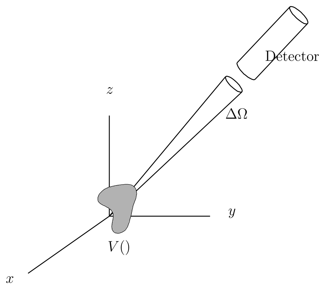
Figure 3:A particle detector intercepts a small solid angle which defines a cone as seen from the scatterer. Particles scattered into this cone will enter the detector.
Cross s and differential cross s were defined in 34. Time-Dependent Perturbation Theory, where the relation between cross s and transition rates was discussed. In the present case let us imagine an experimental situation such as illustrated in Figure 3. A detector, located at some distance from the scatterer, intercepts all scattered particles coming out in a small cone of solid angle , centered on some direction . The counting rate is the scattered current integrated across the aperture to the detector.
The particle density in the incident beam is
Similarly, the incident current is
where is the velocity of the incident beam. In magnitude, .
By our calculation is dimensionless, and if you are fastidious you might want it to have dimensions of inverse volume (or particles per unit volume). If so you can multiply the wave function by a constant of dimensions , but since the physical quantities we are interested in are independent of the normalization of the wave function, this is not necessary.
As for the scattered current, in the asymptotic region it is
which is only an asymptotic form since we are using the asymptotic form (5) of the scattered wave. To evaluate this we take the gradient of the scattered wave spherical coordinates (see (20),
where we only carry the result to leading order in . Substituting this into (8), we find
To leading order, the asymptotic form of the scattered current is purely in the outward radial direction, as we expect. Terms in that go to zero faster than as will not contribute to the counting rate, since the area of the aperture of the detector, for fixed , is proportional to .
Now we integrate the scattered current over the aperture to the detector, which we assume is at large distance from the scatterer, and which has area . The counting rate is
where is the area element of the aperture and is the counting rate per unit solid angle. Now dividing this by , we obtain
a simple result. This equation explains the interest in finding , since it leads immediately to the differential cross , which is measurable. Notice that the counting rate, which is physically observable in a scattering experiment, depends only on the leading asymptotic form of the scattered wave function. One does not need to know the exact form of the scattered wave (at smaller values of where correction terms to the asymptotic expansion of the scattered wave are important, or in the scattering region where the potential is nonzero).
Now for some comments about this calculation. Notice that we computed the flux of the scattered particles intercepted by the detector, but we ignored the incident particles. In realistic scattering experiments the detector is usually located outside the beam, so incident particles do not enter it. Our incident wave (4) fills all of space, but that is an artifact of our model. In reality the beam will be cut off at some finite transverse size, and if the scattering angle is not too small, the detector can be located outside the beam.
If the scattering angle is very small, however, then the detector will have to be inside the beam and it will detect incident particles as well as scattered ones. The counting rate is still the particle flux intercepted by the aperture of the detector, but the flux is neither the incident flux nor the scattered flux nor the sum of the two, but rather the flux computed from the total wave function . Since the current is quadratic in the wave function, there are cross terms or interference terms between the incident wave and the scattered wave. Taking all these effects into account leads to the optical theorem, which we take up in The Optical Theorem.
Central Force Scattering
We now specialize to the important case of a central force potential, . The main simplification in this case is that the Schr"odinger equation (1) is separable in spherical coordinates (see 16. Central Force Motion), so the solutions can be written in the form
where is a solution of version one of the radial Schr"odinger equation, (7), with potential . The radial eigenfunction is parameterized by because the radial Schr"odinger equation contains in the centrifugal potential. It is also parameterized by the energy , which we will normally indicate by an equivalent wave number , given by . The three-dimensional solution depends on , and , as indicated in (16). Of these, is a continuous index and and are discrete.
The solutions (16) of the Schr"odinger equation do not satisfy the boundary conditions (3)--(5) that we require for a scattering solution, but they do form a complete set so the desired scattering solution can be expressed as a linear combination of them. Since the scattering solution is an energy eigenfunction of energy it can only be a linear combination of central force eigenfunctions (16) with the same energy, that is, there must be coefficients such that
where the on the left and the on the right are related by . In a moment we will find the expansion coefficients in terms of some simple parameters that characterize the potential (namely, the phase shifts ).
Free Particle Solutions
Free particle solutions were discussed in Secs. Free Particle{} --WKB Theory and Spherical Bessel Functions. Here we recall some of that material and present some further facts that will be useful in scattering theory.
In the case of the free particle the radial Schr"odinger equation (7) with energy has two linearly independent solutions, and , where and are the spherical Bessel functions. The small and large argument limiting forms of these Bessel functions are given by (27)--(30). If the potential is zero all the way down to , that is, if the particle is free everywhere, then the -type Bessel functions are not allowed because they diverge at . Then a complete set of free particle energy eigenfunctions is
But if we are seeking free particle solutions in some region away from , such as in the asymptotic region of a scattering problem where the potential can be ignored, then the -type solutions are also allowed.
The incident plane wave is a free particle solution of the Schr"odinger equation that is obtained by separating the wave equation in rectangular coordinates, while the solutions (18) are obtained by separating in spherical coordinates. Thus the incident plane wave can be expressed as a linear combination of the solutions (18). The expansion gives as a linear combination of the solutions (18) with the same energy. The expansion coefficients can be worked out with some use of recursion relations satisfied by the spherical Bessel functions and the Legendre polynomials. We omit details here, which may be found in textbooks such as Messiah, Sakurai or Commins. The result, however, is useful. It is
where and refer to the directions of the vectors and on the left hand side, where means the same as and where as usual .
This expansion can be rewritten with the use of the addition theorem for spherical harmonics, (72), which for present purposes we write in the form
where is the angle between and . Then the expansion (19) becomes
Notice that if we take to lie in the -direction, , then is the same as , the usual spherical coordinate. In that case, the incident plane wave becomes
that is, it is independent of the azimuthal angle , and the sum (21) is the expansion of the plane wave in Legendre polynomials of .
The spherical Bessel functions and are real, but complex linear combinations of them are often useful. These are the spherical Hankel functions, defined by
The two types of spherical Hankel functions are complex conjugates of each other,
These functions have particularly simple asymptotic forms when , namely,
which are equivalent to (29)--(30). The phases that makes these expressions look complicated are just conventions. Otherwise the asymptotic forms of the spherical Hankel functions are just , corresponding in scattering problems to incoming and outgoing spherical waves.
Partial Waves
The exact solution of the Schr"odinger equation is decomposed into incident and scattered waves according to
as in (3). The angular dependence of the total wave and that of the incident wave are represented as linear combinations of 's by (17) and (19), respectively. Let us similarly decompose the angular dependence of the scattered wave by writing
where the functions are effectively the radial wave functions of the scattered wave,
Then (26) can be written
This equation is exact. But the 's are linearly independent so (29) is equivalent to
Now we extract the leading asymptotic forms of the three terms in (30) as . As for the total wave function, we need the asymptotic form of . We argue that if falls off rapidly enough then at large it can be ignored and must be a linear combination of the free particle solutions and . Precisely how fast must fall off for this to be true is examined in Asymptotic Form of the Radial Wave Functions. Actually, it is more convenient to use the spherical Hankel functions and to write
where and are the coefficients of the linear combination. Here we are assuming that the exact radial wave function has been chosen to be real, as we can do since the radial wave equation is a real equation. This means that the coefficients of the linear combination of the spherical Hankel functions must be complex conjugates of each other, as shown, because of (24). Thus the phase of is specified to within a ± sign, but its normalization has not been specified. The right-hand side of (31) is a good approximation to the left-hand side when is large enough that the potential can be neglected.
We now break into its magnitude and phase,
and absorb the magnitude into the normalization of . This fixes the normalization of the radial wave functions; they are now determined to within a ± sign. Then we have
or, if we replace the Hankel functions by their asymptotic forms (25), valid when ,
This is the asymptotic form of the radial wave functions; it is parameterized by the phase shifts , which play a fundamental role in central force scattering.
As for the incident wave in (30), it is a plane wave whose radial wave functions are the Bessel functions . These have the asymptotic form
which follows from (23) and (25).
Finally, for the scattered wave in (30) we use (5) in (28) to obtain
where the are the expansion coefficients of the scattering amplitude when expanded as a linear combination of 's,
Altogether, when we take the leading asymptotic form of all three terms in (30) we obtain
All three terms go as at large , so we have obtained the leading asymptotic term of the entire equation (30), and this is exact. The result is a linear combination of incoming and outgoing spherical waves, which are linearly independent; notice that that the scattered wave only has an outgoing part (this is the boundary condition imposed by the physics).
Working first with the coefficients of the incoming wave we see that we can solve for the coefficients in terms of the phase shifts. We find
Then using this in the outgoing part, we can solve for the expansion coefficients of the scattering amplitude. In the algebra it helps to notice that
Thus we find
or,
This is the desired result, which expresses the scattering amplitude in terms of the phase shifts . Another version is obtained with the help of the addition theorem (20),
where we have set so that , where is the usual spherical angle. When it is obvious that the whole central force scattering problem is symmetric under rotations about the -axis so must be a function of alone. Expressions (42) or (43) are the partial wave expansion of the scattering amplitude. We shall discuss this result momentarily, but first we examine an important point that we have glossed over so far.
Asymptotic Form of the Radial Wave Functions
In the derivation of the partial wave expansion we assumed [see (31)] that if the potential dies off rapidly enough with distance, then at large distances the radial eigenfunctions approach linear combinations of free particle solutions. Let us now examine how rapidly must die off for this to be true.
As explained in 16. Central Force Motion, the radial eigenfunction is related to an alternative version of the radial eigenfunction , which satisfies version two of the radial Schr"odinger equation, (11). (Function was called in 16. Central Force Motion.) For our present purposes we rearrange these two versions of the radial Schr"odinger equation as
and
where
Since both the true potential and the centrifugal potential go to zero as , the function also goes to zero as . So as a first stab at analyzing the asymptotic form of , let us neglect altogether on the right hand side of the radial Schr"odinger equation (45). Then the solution for is simply a linear combination of the exponentials , and is a linear combination of , as we assumed in (34).
To take into account the effects of , let us write the solution of (45) as
where is a correction that will account for the effects of the function . If we can show that as , then the correct asymptotic forms of will be a linear combination of the solutions . That is, the function on the right hand side will make no difference in the asymptotic form of the solution. Substituting (47) into the radial Schr"odinger equation (45), we obtain an equation for ,
This is rigorously equivalent to (45).
Now we consider the behavior of as . If the true potential goes to zero faster than , then is dominated by the centrifugal potential and also goes to zero as . We assume , so the centrifugal potential does not vanish. If the true potential goes to zero more slowly than , let us assume that it does so as a power law, , where . This excludes the case of the Coulomb potential, for which , but it approaches the Coulomb potential as . Then has the asymptotic form,
where and is a constant. The case can be handled as a special case, but it does not change any of the conclusions that we shall draw.
We are interested in solving (48) in the asymptotic region when has the asymptotic behavior (49). Let us assume that is asymptotically given by a power law,
where is another constant and . Then the three terms on the left hand side of (48) go as , and , in that order. The third term dominates, so to leading order we have , so that , and the power law ansatz for has a solution. That is, , does go to zero as , and thus the asymptotic form of is a linear combination of .
But in the case of the Coulomb potential, , that is, with . Then taking the dominant term in (48), we have
or,
The logarithm does not go to zero as , in fact, it increases without bound (although very slowly). Thus, in the case of the Coulomb potential, the asymptotic form of the radial wave function is
The Coulomb potential gives rise to long range, logarithmic phase shifts that do not approach the free particle phases as .
In summary, if the potential goes to zero faster than , then the asymptotic form of the radial wave function is given by the linear combinations (for ) or by (for ), the latter of which is what we assumed in the derivation of the partial wave expansion (42) or (43). For the rest of these notes we will assume that does satisfy this condition, thereby excluding the Coulomb potential.
By the way, the derivation of (30) did not make any assumption about the asymptotic behavior of , but now we have shown that if faster than then , so in that case has the same behavior. Then if we choose outgoing boundary conditions we obtain the form (5) for the scattered wave. In the case of the Coulomb potential, however, the form (5) of the scattered wave is not correct.
Partial Wave Expansion of the Cross Section
We return to the partial wave expansion of the scattering amplitude, (42) or (43), which give the scattering amplitude as a linear combination of spherical harmonics or Legendre polynomials. Squaring the scattering amplitude we obtain the differential cross ,
or, with ,
These expressions have cross terms that do not simplify, but which show up experimentally as oscillations in the angular dependence of the differential cross . Some of these may be seen in Figs.~Figure 8 or Figure 9.
On the other hand, when we integrate over all angles to obtain the total cross , the cross terms integrate to zero. This is easiest to see in the form (54), due to the orthonormality of the 's. The result is
or, with another application of the addition theorem (and noting that and ),
This is the partial wave expansion of the total cross .
The Phase Shifts 
These results show the importance of the phase shifts , which determine the coefficients of the angular expansion of the scattering amplitude and cross . We now make some comments on the properties and intuitive meaning of these phase shifts.
The phase shifts are defined by the asymptotic form of the radial wave functions (34) and are determined by the potential . That is, is the phase of the incoming or outgoing part of the exact radial wave function, relative to that of a free particle. Thus, the phase shifts vanish for a free particle. The phase shifts depend on because the radial wave function does so. They depend on the energy, too, and if we wish to emphasize this we can write . Since by our analysis the phase of the radial wave is determined to within a ± sign, the phase shift is determined to within an integer multiple of .
For an intuitive view of the phase shifts we can imagine launching spherical waves inward at the scatterer from a large distance, allowing them to converge on the origin and then bounce back. The wave can be given an angular modulation proportional to a to give it a dependence on . Then we will find a certain phase shift in the reflected wave compared to the incident wave. We can do this both for the free particle and the one with a potential; the difference in the phase shifts in the two cases is .
As a more practical matter, the phase shifts can be determined by solving the radial wave equation somehow and then comparing the asymptotic form of the solution with the form (34) to get the phase shifts. In some cases this can be done analytically, and it can also be done numerically. For the latter one simply chooses regular boundary conditions for at , and then integrates the radial Schr"odinger equation outward numerically. When a radius is reached where the potential is negligible a comparison of the numerical solution to (33) gives the phase shifts. Another approach is to use WKB theory; since the radial wave equation is one-dimensional, WKB theory can be very effective in obtaining information about the radial wave function. Some aspects of this approach were explored in Prob. Paragraph.
WKB theory leads easily to some general conclusions about the phase shifts. Suppose we have a well localized potential, for example, one that dies off exponentially with such as the Yukawa potential (122). Let be a measure of the range of the potential. Then the centrifugal potential, which only falls off as , will dominate for large if . Thus for a given , if is big enough the radial turning point in the centrifugal potential will lie outside the range of the true potential, and the radial wave function will be able to reach the true potential only by tunneling through the centrifugal potential. The wave function decays exponentially in the classically forbidden region, so for such large values the true potential will have only an exponentially small influence on the wave function, which will be nearly the same as a free particle radial wave function of the same value of and . Thus for such large values we expect the phase shifts to be small, and to decay exponentially with as increases beyond a certain cutoff.
To estimate the value beyond which such behavior holds, we set the nominal turning point in the centrifugal potential to the range of the true potential, that is,
If we ignore the difference between and , this gives the estimate,
beyond which the phase shifts decay exponentially toward . In summary, for a well localized potential of range , an estimate of the number of terms that contribute significantly to the partial wave expansion is .
This means that for well localized potentials such as the Yukawa potential, the partial wave sum (57) converges, and the total cross is finite. A more careful WKB analysis is capable of giving more precise conditions on the potential for the total cross to be finite.
Hard Sphere Scattering
As an example of the partial wave expansion, let us consider scattering from a hard sphere. The potential is
where is the radius of the sphere. In the region the solution is a linear combination of free particle solutions, which we write as
which is the same as (31) except for the hard sphere it is exact and (31) was only an asymptotic form. As in the analysis of (31) we write and absorb into the normalization of the , so that are the phase shifts.
These are determined by imposing the boundary condition that vanish at the surface of the sphere,
or,
This can be solved for the , which give us the scattering amplitude and differential cross . We will consider two limiting cases, in which the limiting forms of the spherical Bessel functions can be used.
The limit 
In the first case we assume . This is equivalent to , where is the wavelength of the incident waves, that is, the scatterer is much smaller than a wavelength. The small argument forms of and , (27) and (28), show that in this case is large and negative and is small and positive. We write (63) as
valid when is small, as here. Thus we find, to a good approximation,
Since , this shows that not only is the lowest phase shift small, the higher phase shifts for are even smaller. In this limit
and the series (43) for the scattering amplitude is dominated by the single term . Thus we have
since and . We see that the differential cross is independent of angle,
and the total cross is
The total cross is four times as large as the geometrical cross-al area of the small sphere. The classical cross is just this cross-al area, , but the regime is the one in which we expect classical mechanics to be a poor approximation to quantum mechanics, so we should not be surprised by the difference.
-wave Scattering
When the partial wave dominates the expansion of the scattering amplitude, we speak of -wave scattering. The scattered wave is isotropic and has an equal intensity in all directions, including the forward direction. Since the sphere is too small to create a shadow; instead, the incident wave effectively wraps all the way around the scatterer. As we will see later, -wave scattering applies to any localized potential whose characteristic size satisfies , that is, (not just hard spheres). The fundamental reason was given in The Phase Shifts : for the radial wave functions must tunnel through the centrifugal potential to reach the scatterer, and the tunneling is deeper the higher the value. We see from (65) that when the phase shifts are indeed an exponentially decreasing function of (in fact, including the factorials, even faster than exponential).
There are many physical examples in which -wave scattering is important. For example, a Bose-Einstein condensate is a dilute gas of atoms at a temperature at which the de~Broglie wavelength of the atoms due to their thermal motion is larger than the interparticle separation. Since the gas is dilute, the interparticle separation in turn is much larger than the atomic size, call it , so we have , or . Thus the interactions of the atoms with one another is described by -wave scattering, and scattering of atoms by atoms, in all its complexity, is described by a single parameter, which is the phase shift .
In -wave scattering any two potentials that give the same phase shift will have the same effect. Therefore in theoretical models the exact potential can be replaced by a simpler one, as long as the phase shift is the same. Delta function potentials are popular for this purpose, which explains their appearance in the models of Bose-Einstein condensates such as the Gross-Pitaevski equation (for which see Prob. Paragraph).
When light scatters from particles that are much smaller than the wavelength, for example, when optical radiation is scattered by atoms in a gas, is this -wave scattering, and is the scattered wave isotropic? (This is a tricky question.) The answer is no, because electromagnetic waves are vector waves, not scalar waves as we have been discussing in these notes. In the case of electromagnetic waves, the scattering when is dominated by dipole radiation, which has a nontrivial angular dependence. Electromagnetic waves have no monopole radiation (that is, -wave radiation), and the next higher term in the multipole series is the first one to appear. It is the one that dominates at small .
Similarly, gravitational radiation, which has received much attention since its actual detection a few years ago, has neither a monopole nor a dipole term, rather the first multipole to appear is the quadrupole.
The Limit 
The second case we consider is the opposite extreme, , that is, . In this case the sphere is much larger than a wavelength. Now there are many values that contribute to the partial wave sum. For small , for which , we can use the asymptotic forms (25) in (63). We find
or, with ,
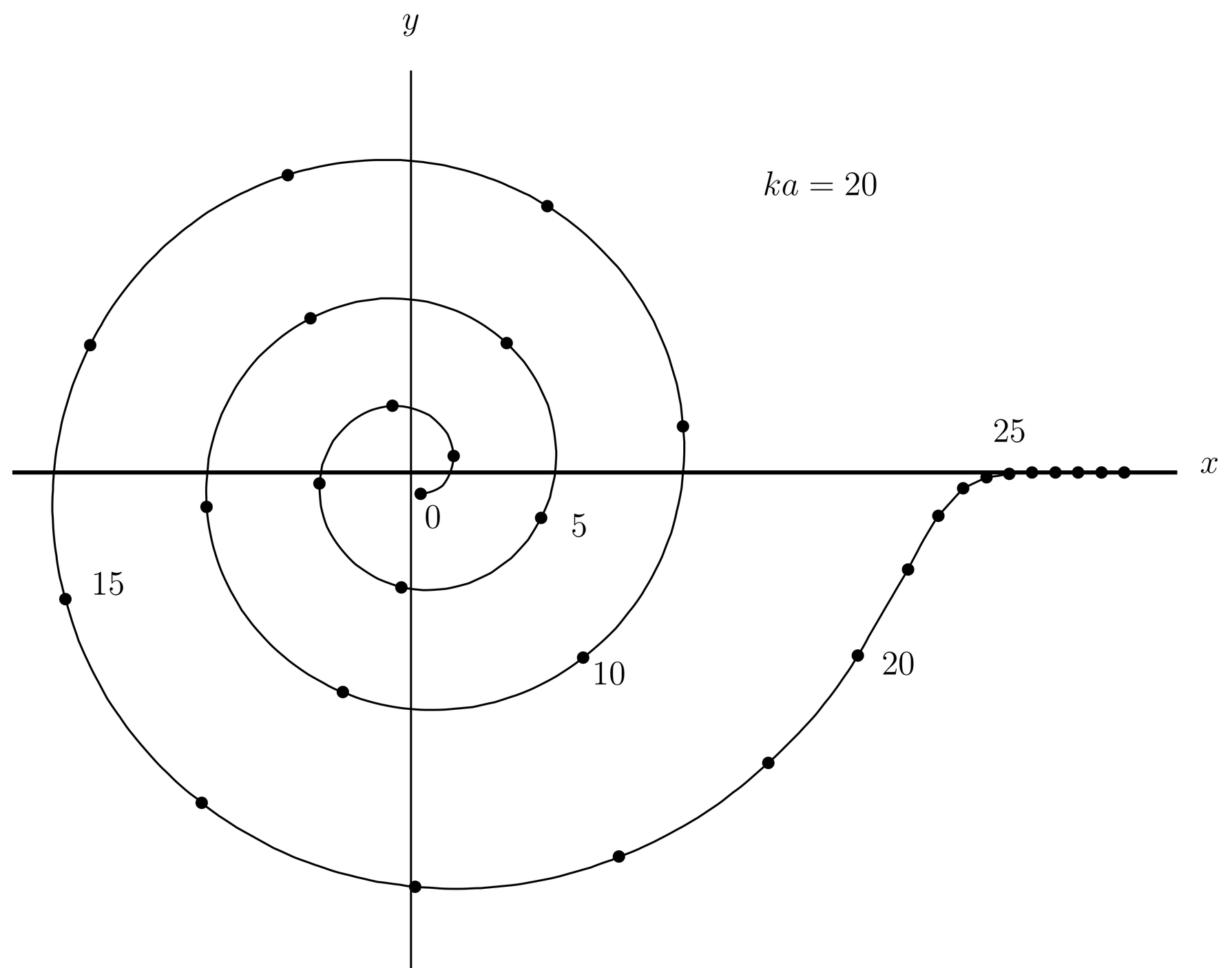
This says that advances by when increases by 1, but this is an approximation that is only valid when . According to (59) we need to sum the partial wave expansion out to , after which we expect the terms of the series to rapidly approach zero. Actually the increment in , which is indeed when , gradually decreases as climbs toward , after which it rapidly goes to zero. This behavior is illustrated in some numerical examples in Figs.~Figure 4 and Figure 5.
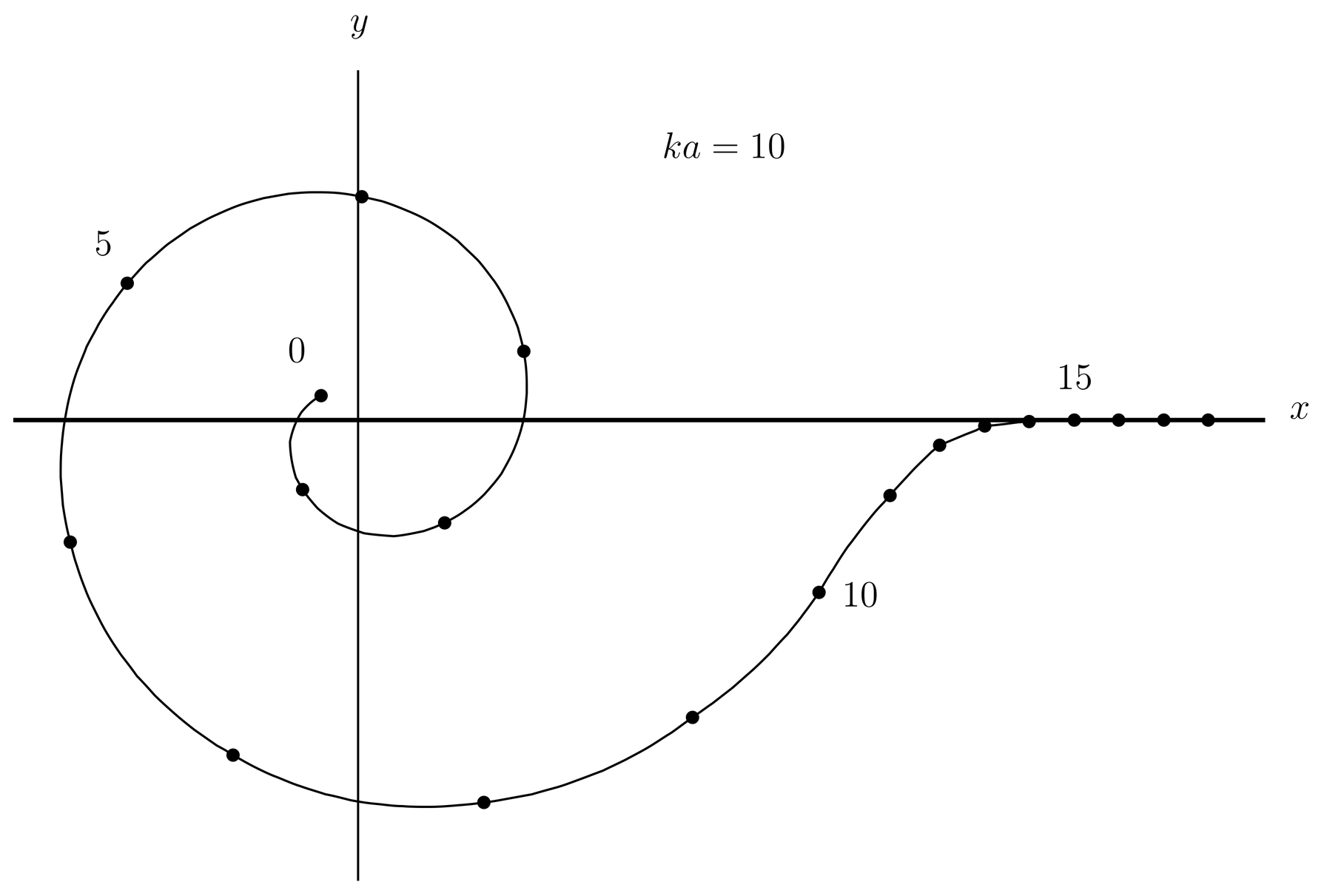
Figure 4:Phase shifts in hard sphere scattering. The phase shifts are represented as points on a circle with plane polar angle . The radius of the circle grows as increases, to keep the points from getting mixed up with each other as they orbit the circle. Some points are labeled with their values. The phase shifts increase with decreasing increment as increases, until , whereupon . Plot is for .
The cutoff at was explained earlier in terms of WKB theory; a more intuitive explanation is illustrated in Figure 6. We imagine particles of fixed energy emitted in various directions from a point on the surface of a sphere of radius . These represent the waves scattered by the sphere. The angular momentum of the particles depends on the direction of emission; its minimum value is when the particles are launched in the radial direction, and its maximum value is when the particles are launched tangentially to the sphere. The maximum value of corresponds to a maximum angular momentum quantum number, . The same reasoning works for any short-range potential with an effective range of ; the partial wave expansion cuts off near .
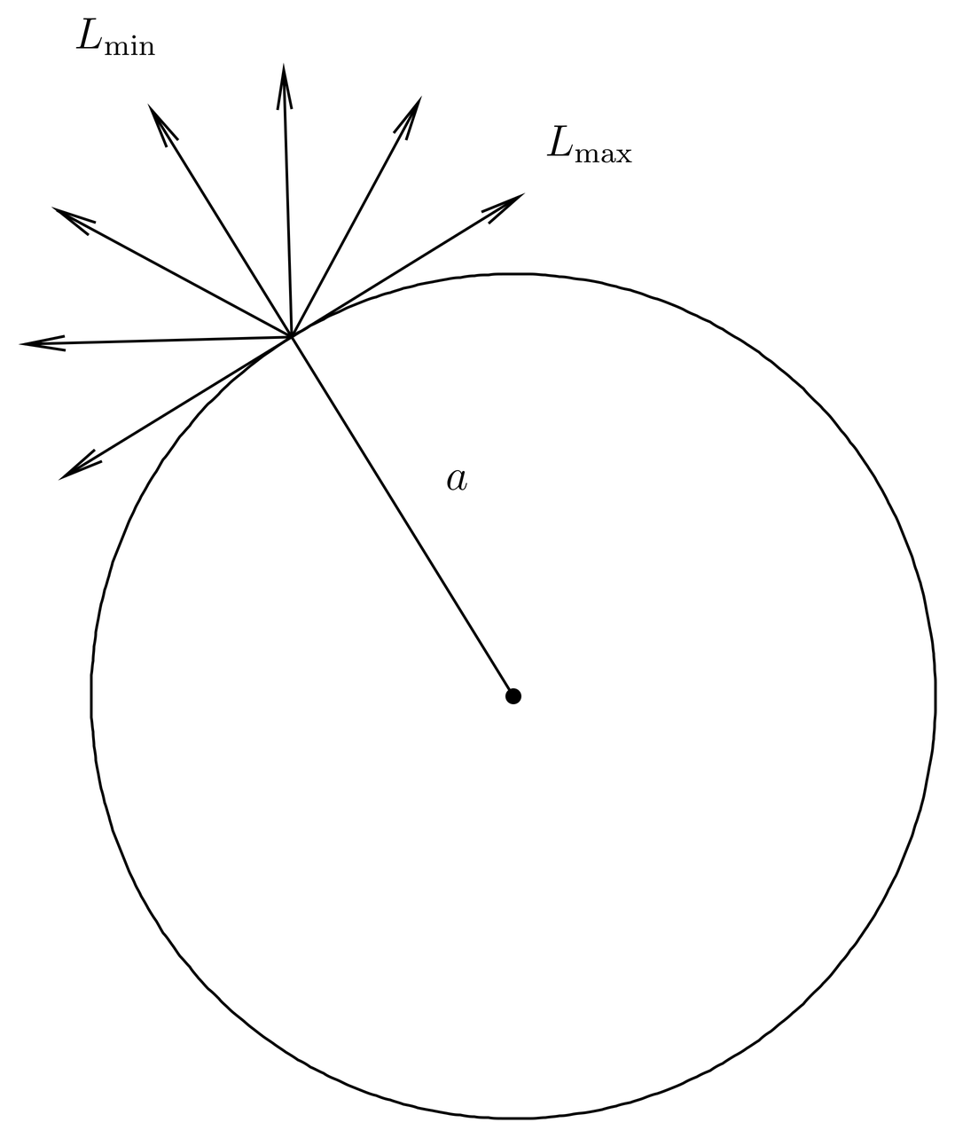
Figure 6:Particles of fixed energy are launched in various directions from a point on the surface of a sphere. The maximum angular momentum is achieved when the direction is tangent to the sphere at the point of launch.
We can use the behavior of the phase shifts to estimate the total cross in the limit . While the points representing the are orbiting their circle as in Figs.~Figure 4 and Figure 5, the average value of is . Since the series cuts off near , the total cross (57) can be estimated by
Using the sum
we obtain the estimate
where we ignore the difference between and . We see that the cross is twice the classical value in the case .
These conclusions are confirmed by detailed calculations, which show that as and as . See Figure 7.
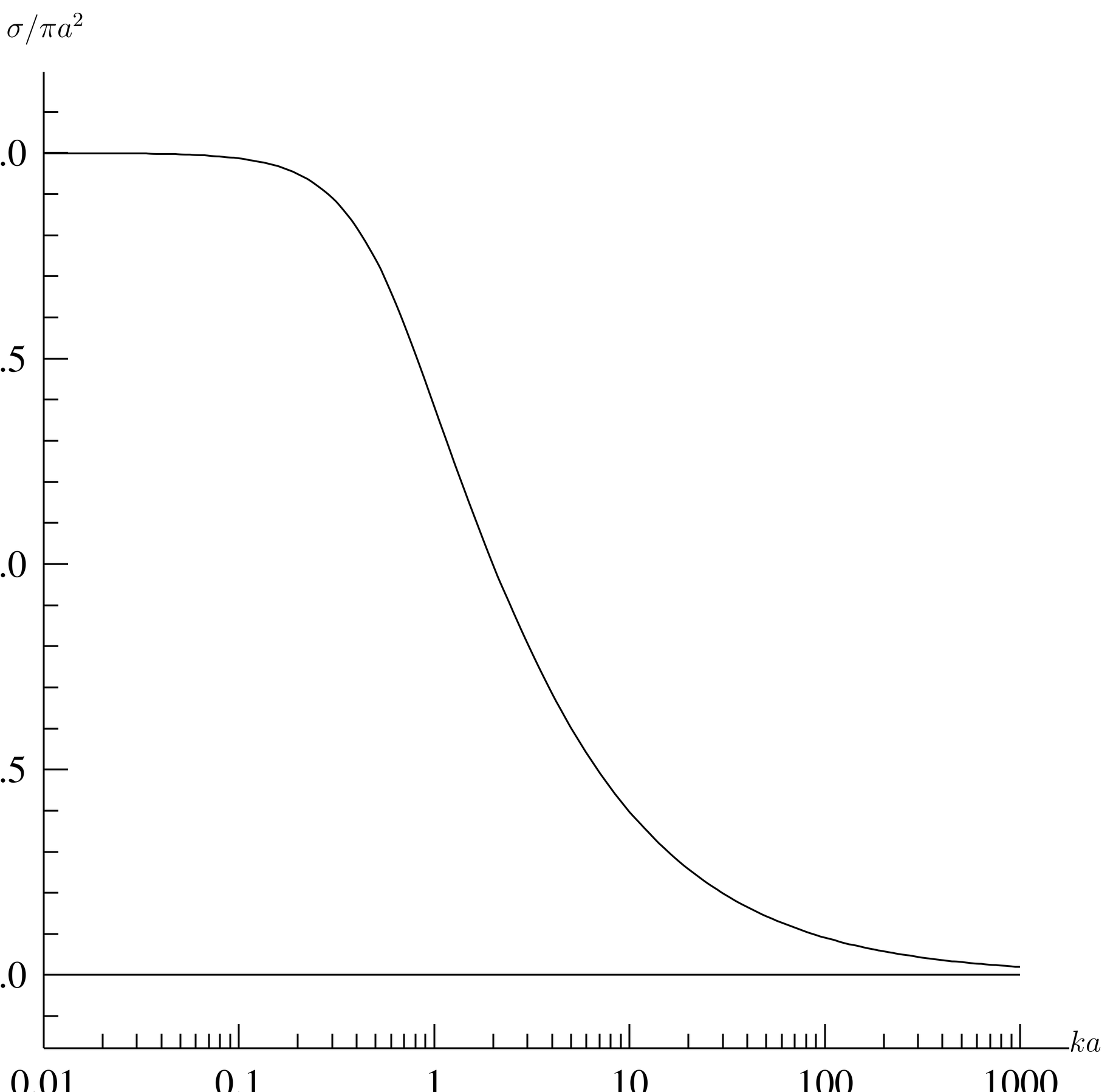
Figure 7:Total cross as a multiple of for hard sphere scattering as a function of . The total cross has the limits as and as .
If we think of the classical limit as one in which the de~Broglie wavelength is much smaller than the scale of the potential, then it is surprising that the limit as since this is twice the classical cross , . To see how this “extra” cross-is distributed in angle we refer to Figure 8, a plot of the differential cross for various values of .
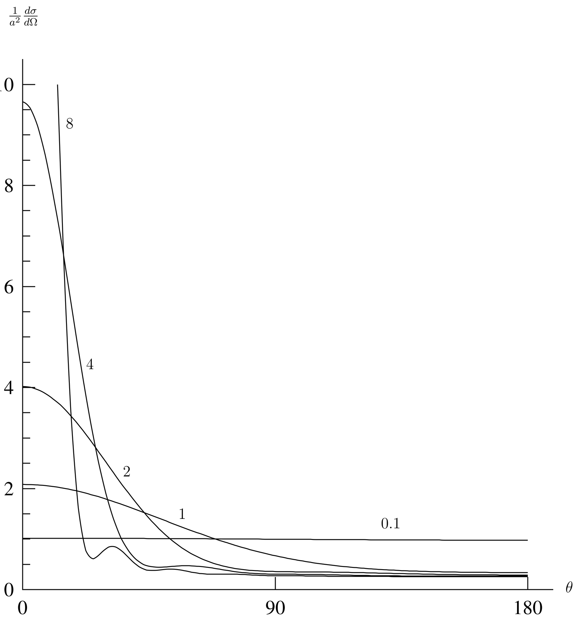
Figure 8:Differential cross in hard sphere scattering, as a multiple of . Curves are labeled by the value of , which increases from 0.1 to 8. Scattering angle is measured in degrees.
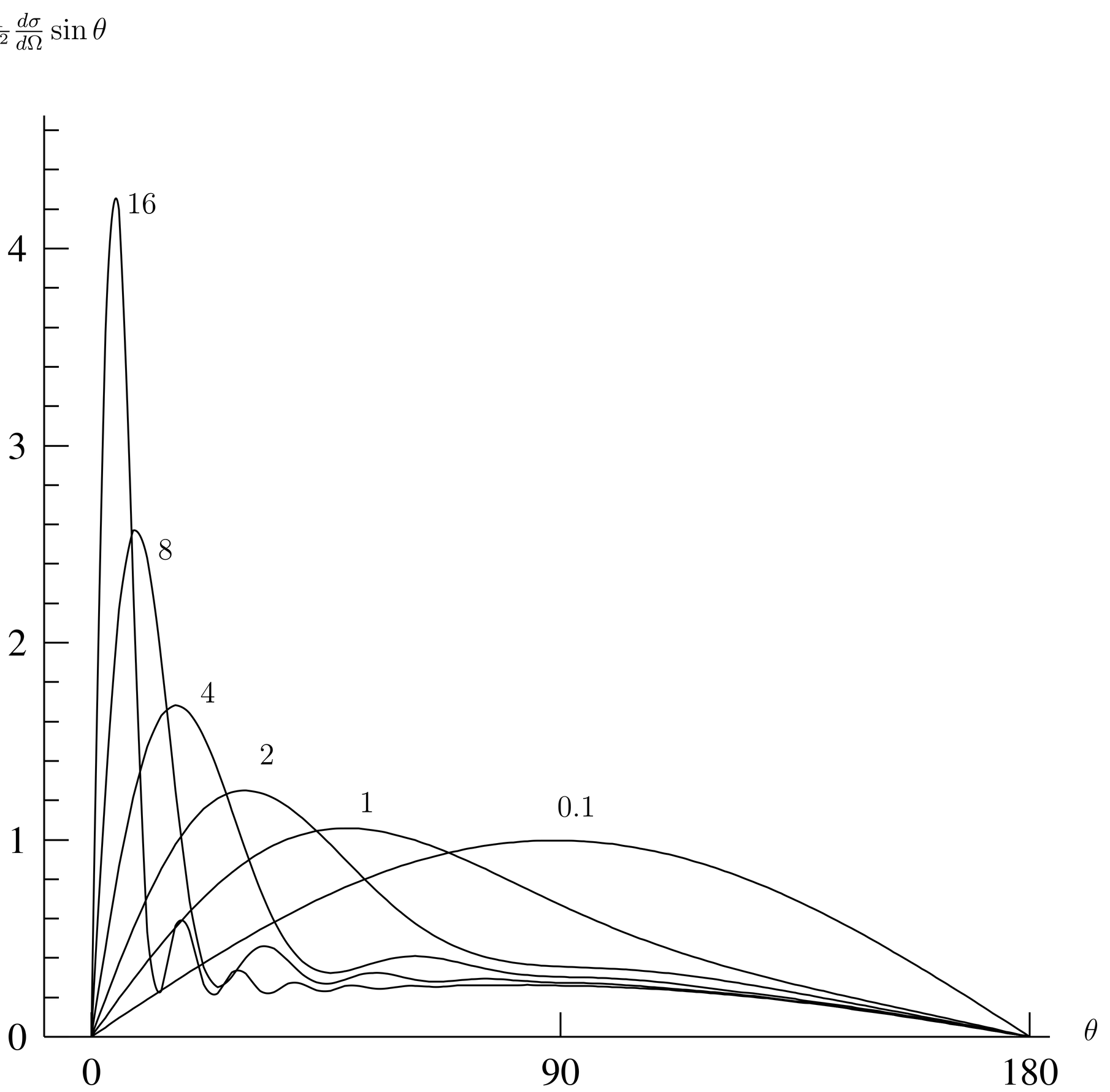
Figure 9:Same as Figure 8 except multiplied by . Area under curves in a given angle range is proportional to the total cross in that range.
Figure 8 shows that for small values of , the differential cross is nearly independent of angle, confirming that we have -wave scattering. The cross is nearly in this range, confirming (68). As increases, decreases at large angles toward the classical value, but at small angles a forward peak rises up, growing narrower and higher. At the edge of forward peak there also arise oscillations. Figure 9 is a similar plot except that has been multiplied by , which makes the integrated cross proportional to area under the curve. This makes it easier to see that the total cross in the forward peak is about the same as the classical cross . In fact, detailed calculations (see Prob.~\prbrintroscatt-1) show that both the forward peak and the classical cross contribute to the total. The “extra” cross comes entirely from the forward peak.
This peak is due to diffraction. As the waves pass by the edge of the sphere they are bent in an inward direction, that is, the direction necessary to close in the shadow behind the sphere. Diffraction theory shows that if we move far enough downstream, the shadow is completely filled by diffracted waves. Of course the differential cross is defined in the limit , so there is no shadow in the differential cross . Diffraction causes the direction of the waves to change from the incident direction, and so must be counted as part of the scattering.
The Optical Theorem
The optical theorem is an exact relationship between the total cross and the scattering amplitude . In the context of potential scattering that we have considered in these notes, the optical theorem is
where refers to the scattering amplitude in the forward direction.
The optical theorem is trivial to prove in the case of scattering by central force potentials. We place the -axis along the direction of the beam so that the usual polar angle is the scattering angle. Then (43) implies
where we have used (57) and (76). This proof is straightforward but it gives no insight into what the theorem means.
The theorem (75) actually applies to scattering by any potential that dies off faster than as , so that the asymptotic wave function is
as indicated by (3) and (5). That is, we need not assume that the potential is rotationally invariant. The two terms in (77) are the incident and scattered waves, respectively.
Since the wave function is a solution of the time-independent Schr"odinger equation, the current
satisfies , so by Stokes’ theorem the integral of over any closed surface vanishes. See (55)--(57). We will integrate over a large sphere of radius centered at the origin of the coordinates, which we assume is inside the region occupied by the potential as in Figure 2. We will take the limit , so that the asymptotic form (77) of the wave function can be used.
Thus the asymptotic form of the current is
where we have set and and retained only the leading term in the gradient of the scattered wave, as in (12). The neglected terms will not contribute to the integral over the sphere when we take the limit .
The current is quadratic in the wave function , so in addition to the incident current and scattered current there is a contribution coming from the cross terms, which represent the interference between the incident wave and the scattered wave. We write
where is the interference current. By Stokes’ theorem we have
where is the area element of the sphere.
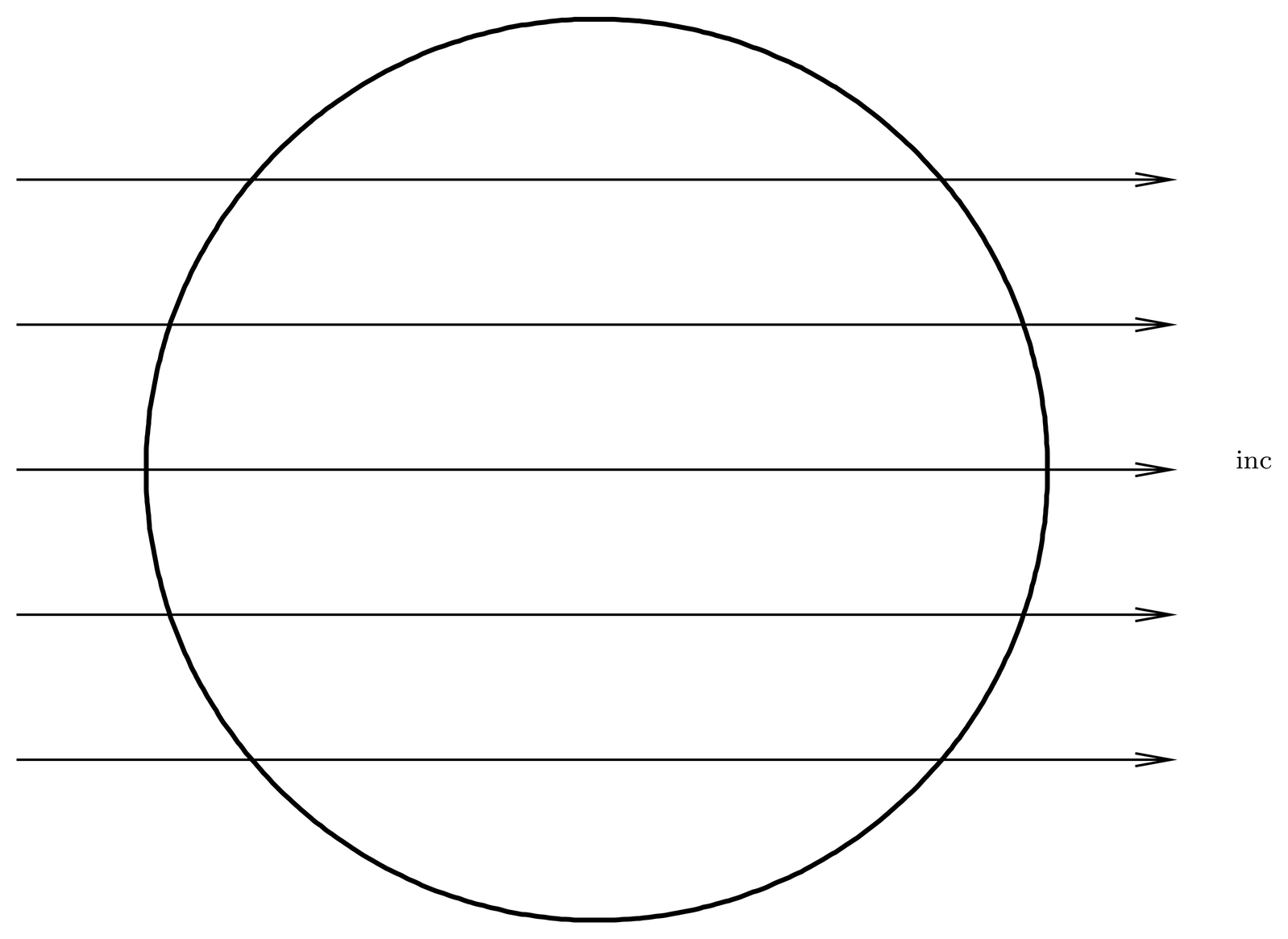
Figure 10:The incident current passes straight through the sphere and produces no net flux across its surface.
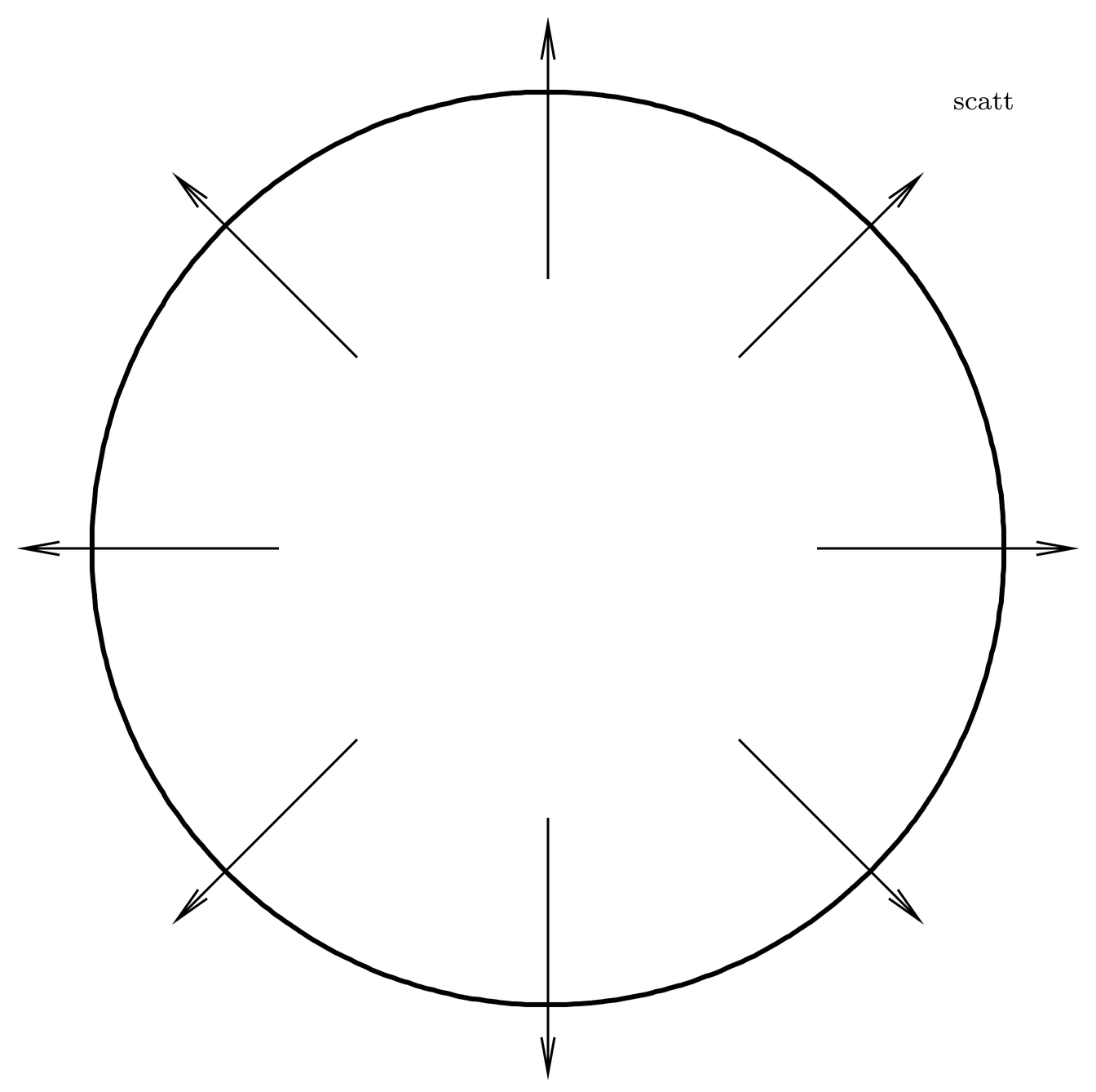
Figure 11:The scattered current produces a net flux of particles leaving the sphere, proportional to the total cross .
The incident current is
It is a constant vector whose integral over sphere vanishes,
as is obvious from Figure 10.
The scattered current was already computed in The Scattering Amplitude and Cross Section. It is
whose integral over the sphere is
where is the total cross and where we have used (15). The scattered wave gives a net outgoing flux, proportional to the cross , which is no surprise. See Figure 11.
Therefore the interference current must provide a net inward flux that cancels the scattered flux. From (79) we have
But the real part of a complex number is the same as the real part of its complex conjugate, so we can replace the first term in (86) by its complex conjugate to obtain
Now the interference flux is
We wish to evaluate this integral in the limit , which is slightly delicate. The prefactor of would tend to make the integral diverge, but the factor in the integrand oscillates ever more rapidly in as gets larger, thereby chopping up the integrand and tending to make the integral vanish. To clarify the competition between these tendencies, we integrate by parts in , obtaining
The integration by parts has eliminated the prefactor of , so now the final integral oscillates itself to death as and can be dropped. Evaluating the remaining term under the -integral at the limits , we see that it vanishes at and that at it is proportional to which is what we are writing simply as and which is independent of . Thus we find
The sum of this plus the scattered flux vanishes, which produces the optical theorem (75).
We see that the interference flux comes in from the forward direction, where it partially cancels the incident flux going in the other direction.
The optical theorem has many generalizations. One version of it applies for the scattering of classical electromagnetic waves (vector waves, in contrast to the scalar waves considered here). Another applies to inelastic scattering in quantum mechanics, in which is the total cross , including both elastic and inelastic scattering, while refers only to the forward amplitude for elastic scattering. This is because only the wave for elastic scattering can interfere with the incident wave. There are many other applications in fields ranging from quantum mechanics to black hole physics.
Problems
Problem 1.
The strange thing about scattering from a hard sphere in the limit is that the total cross section is , not , the geometrical cross section. When the wave length is short, we expect quantum mechanics to agree with classical mechanics, but it does not in this case.
(a) Work out the classical differential cross for a hard sphere of radius , and integrate it to get the total cross .
(b) In problem Paragraph, you worked out the far field wave function , for , when a plane wave traveling in the positive -direction strikes a screen in the - plane with a circular hole of radius cut out. In that problem the hole was centered on the origin. The solution was worked out for (the paraxial approximation), where .
By subtracting this solution from the incident wave , you get the far field wave function when a plane wave strikes the complementary screen, that is, just a disk of radius at the origin.
It turns out this wave field is the same as the wave field in hard sphere (of radius ) scattering in the limit , if measured in the forward direction. That is because for forward scattering from a hard scatterer, the physics is dominated by diffraction, so it is only the projection of the scatterer onto the - plane that matters.
Write the scattered wave as , express as a function of and for small , expand out to lowest order in , and compare to the asymptotic wave field to get an expression for the scattering amplitude for small angles . Use the optical theorem, (75), to compute .
(c) Show that in the forward direction has a narrow peak of width . Write down an integral giving the contribution of this forward peak to the total cross in terms of the first root of the Bessel function . You can approximate in this integral, since is small. It turns out that the value of this integral does not change much if the upper limit is extended to infinity. Use the integral
to find the contribution of the forward peak to the total cross . (See Gradshteyn and Ryzhik, integral number 6.538.2.)
Problem 2.
This problem is borrowed from Sakurai. Consider a potential
where may be positive or negative. Using the method of partial waves, show that for and the differential cross is isotropic and that the total cross is given by
Suppose the energy is raised slightly. Show that the angular distribution can then be written as
Obtain an approximate expression for .
Problem 3.
This problem is best done after some experience with scattering of particles with spin, such as Problem~Paragraph.
Consider the scattering of a polarized, spin~ particle by a target, such as a neutron by the nucleus of an atom (we may assume that the nucleus is polarized, too). There is some amplitude for scattering that does not flip the spin, and some for scattering that does.
Suppose the incident particle is polarized spin up, so that the incident wave function can be taken to be
The asymptotic form for the scattered wave is
where are the scattering amplitudes with () and without () spin flip.
Find a generalization of the optical theorem in this case. Recall (32) for the probability current for particles with spin. Is it possible that some target could cause the spin to flip with 100% probability? How do your answers change if a magnetization term such as seen in (35) is included in the probability current?