37. Green's Functions in Quantum Mechanics
37. Green’s Functions in Quantum Mechanics
Introduction
Green’s functions and the closely associated Green’s operators are central to any reasonably sophisticated and comprehensive treatment of scattering and decay processes in quantum mechanics. In these notes we shall develop the theory of Green’s functions and operators, which will be applied to simple scattering problems in the next set of notes. Later, in 44. Natural Line Width, Long-Time Behavior and the Lamb Shift, we will see that Green’s operators provide the key to understanding the long-time behavior of quantum systems, such as an atom undergoing radiative decay. Green’s operators are also necessary for the construction of the -matrix, a central object in the most satisfactory treatments of scattering theory, especially in relativistic quantum mechanics.
The Green’s functions and operators that we will deal with come in two varieties, the time-dependent and the energy-dependent (or time-independent). Time-dependent Green’s functions are closely related to the propagator that we studied in 09. The Propagator and the Path Integral. They are useful for solving time-dependent problems, such as the types we treated earlier by time-dependent perturbation theory.
We begin these notes by presenting a sketch of the problem of scattering of electromagnetic waves, which provides a motivation for the use of Green’s functions in scattering theory in general. Next we discuss time-dependent Green’s functions in quantum mechanics, which are a stepping stone into the theory of energy-dependent Green’s functions. We present water wave analogies for both time-dependent and energy-dependent Green’s functions in quantum mechanics, which not only provide useful physical pictures but also make some of the mathematics comprehensible. Finally, we work out the special case of the Green’s function for a free particle. Green’s functions are actually applied to scattering theory in the next set of notes.
Scattering of Electromagnetic Waves
In the following presentation of scattering of electromagnetic waves we shall use only the most schematic notation, suppressing indices , , etc as well as ’s, ’s, etc. The point is to convey the general structure of the equations and the physical picture associated with them without going into details.
We write Maxwell’s equations for the vector potential (really the 4-vector ) in the form
where is the 4-current (really ) and where is the d’Alembertian operator,
(1) holds in Lorenz gauge (). Mathematically, (1) is an inhomogeneous equation, that is, it has source or driving terms (the current) on the right-hand side.
The corresponding homogeneous equation is
with no source term. We put an -subscript on the solution of the homogeneous equation; physically, represents a source-free electromagnetic field, for example, a vacuum, plane light wave. Notice that if we have two solutions of the inhomogeneous (1),
then their difference is a solution of the homogeneous equation,
A common problem in electromagnetic theory is to compute the field produced by a given source current . The standard method for solving such problems uses Green’s functions. The general solution of the inhomogeneous equation (1) is
again in a very schematic notation in which means , and where is a Green’s function for the operator . An arbitrary solution is added to the right-hand side, to give the general solution for . The solution of an inhomogeneous equation is never unique, because one can always add an arbitrary homogeneous solution to it. Physically, a unique solution is selected out by boundary conditions (which allow one to choose the correct ).
The Green’s function satisfies
where acts only on the dependence of . This is itself an inhomogeneous equation, so is not unique, either. Usually different Green’s functions are characterized by the boundary conditions they satisfy.
All of this is for a given , but in practice we may not know ahead of time what is. Consider, for example, the scattering of electromagnetic waves by a metal object. When the incident wave strikes the metal, its electric field causes currents to flow in the metal, and these radiate the scattered wave. More precisely, the electrons in the metal respond both to the incident field and the scattered field, that is, the current elements act on one another as well as responding to the incident field. Thus we have
where is the conductivity operator and is the total field, the incident plus the scattered. (You are probably familiar with the above equation in the form , where is often taken as a constant. But is related to the derivatives of , and in (8) we have absorbed those derivatives into the definition of . Also, is in general not constant, but an operator. (8) is a general statement of the relation between the current and the fields that drive it in a linear medium.) Although responds to the total field, incident plus scattered, it is the source of the scattered wave only.
With the substitution (8), the original equation (1) becomes
or,
The original, inhomogeneous wave equation has become homogeneous. We see that whether an equation is homogeneous or inhomogeneous depends partly on our point of view. We also see that finding the scattered wave is a self-consistent problem of finding sources produced by the incident plus scattered wave that themselves produce the scattered wave.
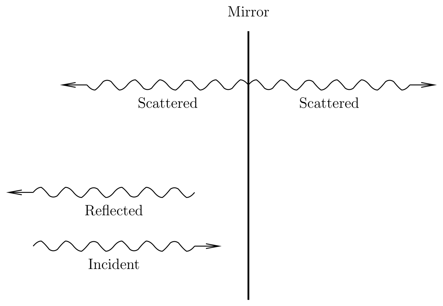
Figure 1:Reflection of light from a mirror. In one point of view we have an incident and a reflected wave, satisfying certain boundary conditions at the surface of the mirror. In another point of view, we have the incident wave plus the scattered wave radiated by currents in the metal.
As a simple example, consider the reflection of light from a mirror. The usual point of view in textbooks is to regard this as a boundary value problem, in which one forms linear combinations of vacuum light waves to the left of the mirror (the incident plus reflected wave, see Figure 1), whose sum satisfies certain boundary conditions at the surface of the mirror. There is no field to the right of the mirror because the wave cannot penetrate it. In another point of view, however, the total field is the incident field which is a vacuum plane wave everywhere in space, including to the right of the mirror, plus the scattered field which is the field produced by the currents in the mirror. These currents radiate in both directions, and they do so in such a manner that the scattered wave to the right exactly cancels the incident wave in that region. It is this latter point of view that will dominate our treatment of scattering theory from here on out.
Sources and Scattered Waves in Quantum Mechanics
The physical picture of currents and sources afforded by electromagnetic scattering can be carried over to quantum mechanics. To be specific, consider potential scattering of a spinless particle in three dimensions, where the Schr"odinger equation we wish to solve is
Here and is the positive energy of some scattering solution. We rearrange this equation in the form,
This should be compared to the electromagnetic equation,
In both cases we have a free particle or free wave operator on the left-hand side, in the electromagnetic case and in the quantum case. On the right-hand side we have a term proportional to the field, in the electromagnetic case and in the quantum case. We see that the potential plays the same role as the conductivity in the electromagnetic case. The wave function can be seen as the sum of an incident plus a scattered wave, in which the scattered wave is produced by “sources” whose “strength” at any point is .
To solve (12) we require a Green’s function for the operator , which is an example of an energy-dependent Green’s function. Before discussing energy-dependent Green’s functions, however, we must first discuss time-dependent Green’s functions.
Time-Dependent Green’s Functions in Quantum Mechanics
Let us consider the inhomogeneous time-dependent Schr"odinger equation,
where is some Hamiltonian and is a “source” term. We allow the Hamiltonian to depend on time because sometimes it does and in any case it leads to the most symmetrical treatment of the problem. Later we will specialize to the case of time-independent Hamiltonians. To solve this equation we require a time-dependent Green’s function , that is, a function that satisfies the equation
Any function that satisfies this differential equation will be considered a Green’s function for the operator . The Green’s function depends on a pair of space-time points. We will think of the first of these, , as the “field” point, and the second, , as the “source” point. But be careful, because some books (for example, Jackson’s) reverse these interpretations, sometimes randomly. The Hamiltonian operator only acts on the field variables, for example, if it is a kinetic-plus-potential operator,
then acts on the -dependence of . The on the right-hand side of (15) is conventional. The rest of the right-hand side is obviously a four-dimensional space-time -function of the type we saw in (7).
If we can find such a Green’s function , then the general solution of the inhomogeneous equation (14) can be written,
where is an arbitrary solution of the homogeneous equation,
That is, is a solution of the ordinary (homogeneous) Schr"odinger equation with Hamiltonian (without driving terms). Since there are many such solutions, the solution (17) of the inhomogeneous equation is not unique.
We see that if we can solve the inhomogeneous equation with a -function driving term, that is, (15) for the Green’s function , then we can solve the inhomogeneous equation (14) with an arbitrary driving term. In effect, we break up the driving term into a sum of -function contributions, and then add the wave fields (the Green’s function ) corresponding to each of these. The result is the integral in the second term in (17).
The Outgoing Time-Dependent Green’s Function
There are many time-dependent Green’s functions, but the most important one for our purposes is the outgoing (or retarded) Green’s function, defined by
Here is the Heaviside step function,
which has the property,
Also, in (19) is the time-evolution operator (see The Time-Evolution Operator), which depends on both the final time and the initial time since the Hamiltonian is time-dependent. The properties of that we need are the Schr"odinger equation,
and the initial conditions,
(see Secs. The Time-Evolution Operator and Differential Equations for Time Evolution). The hat on in (22) will be explained momentarily.
To show that actually is a Green’s function, we differentiate both sides of (19), obtaining,
where we have used (22) in the second term. As for the first term on the right-hand side, the -function vanishes if , so we might as well set inside , since the answer vanishes otherwise. But then we can use the initial conditions (23), so the first term becomes
As for the second term, we must first explain that we are using the notation to stand for the Hamiltonian operator acting on wave functions , while writing to stand for the corresponding operator acting on kets. The relation between them is
Thus the second term on the right-hand side of (24) can be written,
Rearranging the result, we have
This proves that is indeed a Green’s function for (14).
In 09. The Propagator and the Path Integral\ we used the notation
(without the subscript) and we called the function the “propagator.” The outgoing Green’s function , related to by
is also called the “propagator,” or, to be more precise, the “outgoing” or “retarded” propagator. The two functions are closely related, but (without the -function) is not a Green’s function.
The properties of that will be important to us are the following. First, vanishes for , on account of the step function. Second, is a solution of the time-dependent Schr"odinger equation in the field variables for , since the function on the right-hand side of (28) vanishes for . It also (trivially) satisfies the Schr"odinger equation for , since in that case. Third, if we let approach from the positive side, then approaches . This follows from the definition (19), since on the positive side, and (the identity operator) in the limit. That is,
Thus, for can be thought of as the solution of the time-dependent Schr"odinger equation with the singular initial conditions at .
These properties allow us to visualize the outgoing Green’s function in a water wave analogy. We imagine a lake that has been quiet from until , whereupon we go to position in the lake and disturb it in a spatially and temporally localized manner (for example, we poke our finger into the lake just once, or throw a stone into the lake). Then the wave field that radiates outward from the disturbance is the outgoing time-dependent Green’s function, that is, is the value of the field at position at time , that was produced by the disturbance at point at time . The waves for are freely propagating (they are not driven).
For another example, an earthquake or an underground explosion is a disturbance that is localized in space and time, and the waves that radiate outward are the outgoing Green’s function for sound waves in the earth.
If we use the outgoing time-dependent Green’s function to solve the driven Schr"odinger equation (14), then the solution is
However, the factor that appears in the definition of means that the integrand vanishes for times , so the upper limit of the integration in the integral (32) can be replaced by . Also, let us impose the requirement of causality, that is, the field is caused by the source . This means that if for times , then we must have for . So setting in (32) to some time , the left hand side vanishes, as does the integral, because the variable of integration must satisfy , so . Therefore the homogeneous solution must also vanish for . But this means that for all , since the solution of the homogeneous equation is determined by its initial conditions, which in this case are zero. Altogether, the causal solution we obtain using the outgoing Green’s function is
where we have dropped the subscript on (see (29), since it is not necessary any more.
This is the causal solution of the inhomogeneous wave equation. It is also possible to construct solutions that do not obey the principle of causality (the wave is nonzero before the source acts). These solutions are nonphysical, but useful in scattering theory nonetheless.
The Incoming Time-Dependent Green’s Function
There is another time-dependent Green’s function of importance, the incoming or advanced Green’s function, defined by
In comparison to the definition (19) of , the argument in the step function is reversed, so vanishes for times . It will be left as an exercise to show that actually is a Green’s function, that is, that it satisfies (15).
The incoming Green’s function satisfies the Schr"odinger equation in the variables both for and , trivially in the latter case since for those times. It also has the limiting form as approaches from below,
Thus, in the water wave analogy, consists of waves that have existed on the lake from time up to . As approaches from below, these waves converge on location , assembling to produce a -function precisely at as . At that instant, our finger comes up and absorbs all the energy in the wave, leaving a quiet lake for all times afterward ().
Obviously the incoming Green’s function would be impossible to set up experimentally, while the outgoing Green’s function is easy. This is why the outgoing Green’s function is the primary one used in scattering theory, where the waves travel outward from the scatterer. Nevertheless, the incoming Green’s function is also important in scattering theory, as we will see.
Green’s Operators
We associate the Green’s functions with Green’s operators by
The Green’s functions are just the position space matrix elements of the Green’s operators, that is, the functions are the kernels of the integral transforms in position space that are needed to carry out the effect of the operators on wave functions. We will write Green’s operators with a hat and Green’s functions without one. The definitions (19) and (34) of the Green’s functions are equivalent to the operator definitions,
These satisfy an operator version of (15),
where the right-hand side is understood to be a multiple of the identity operator. When we sandwich both sides of this between and , the spatial -function appears on the right-hand side, as seen in (15).
The operator notation is not only more compact than the wave function notation, it is also more general, since we do not have to be specific about the form of the Hamiltonian or the nature of the Hilbert space upon which it acts. For example, it applies to particles with spin, multiparticle systems, composite particles with internal structure, relativistic problems, and field theoretic problems of various types.
Time-Independent Hamiltonians
In the special case that is independent of time, the time-evolution operator depends only on the elapsed time (see Differential Equations for Time Evolution). In this case we will write for the time evolution operator, where is now the elapsed time, and of course we have . Then with a slight change of notation we define the operators
which satisfy
We will write
for the Green’s functions in the case of time-independent Hamiltonians.
As a special case, for the free particle in three dimensions, , the Green’s functions are
where the 0-subscript refers to “free particle.” See (13).
Energy-Dependent Green’s Functions in Quantum Mechanics
Let us now consider the inhomogeneous time-independent Schr"odinger equation,
where is a time-independent Hamiltonian and is a source term. As above, stands for the differential operator acting on wave functions , for example,
and stands for the Hamiltonian operator acting on kets. To solve (43) we require a Green’s function for the operator , that is, a function that satisfies
where acts only on the -dependence of (the “field” point), while (the “source” point) and are considered parameters. The Green’s function depends on because the operator depends on ; we shall call it an energy-dependent Green’s function. We will use the symbol for energy-dependent Green’s functions, and for time-dependent Green’s functions. The energy is not necessarily an eigenvalue of the Hamiltonian , rather it should be thought of as a parameter that we adjust depending on the application. In fact, as we shall see shortly, it sometimes even takes on complex values.
Green’s functions are not unique, but if we find one, we can write the general solution of (43) as
where is a solution of the homogeneous equation, . That is, is an eigenfunction of of energy (and if is not an eigenvalue of , then ).
We can express an energy-dependent Green’s function in terms of an associated operator by writing
Then the defining equation (45) of an energy-dependent Green’s function can be written in operator form as
This would seem to have the solution,
but, as we shall see, the operator either has no inverse, or has a unique inverse, or has many inverses, depending on the value of . In a finite-dimensional vector space, an operator (that is a matrix) has an inverse if and only if its determinant is nonzero, and if it has one, it is unique. In infinite dimensional spaces this is no longer true. As we shall see, the multiple inverses that exist for are related to boundary conditions.
The mathematics of energy-dependent Green’s functions is tricky because of various noncommuting limits, which are related to the fact that the Schr"odinger equation has no damping. In the following we make no pretense of mathematical rigor, but we will attempt to provide physical models and images that help visualize the functions being considered and that make their mathematical properties plausible. To start this process, we now make digression into the subject of frequency-dependent Green’s functions for water waves, the analog of energy-dependent Green’s functions in quantum mechanics. This will provide us with concrete physical images and analogies to help us understand the mathematics we will encounter later with quantum mechanical Green’s functions.
A Water Wave Analogy
The analogy between water waves and Schr"odinger waves is imperfect because water waves obey nonlinear differential equations that are second order in time, while the Schr"odinger equation is linear and first order in time. (Small amplitude water waves are governed by a linear equation, however.) We shall gloss over such differences, concentrating instead on the physical picture afforded by the analogy.
Imagine a lake of finite area that has been quiet from until , whereupon we go to position (the source point) in the lake, and create a spatially localized disturbance that is periodic with frequency (for example, we poke our finger up and down in the water). We do this for all positive time from to . As you can imagine, waves are radiated from the initial disturbance, they travel to the shores and reflect and come back, creating a complicated wave pattern that nevertheless simplifies after a while because of the decay of the initial transients. The decay depends on the damping present in the water waves; we assume the damping is small, and represented by a parameter . After the decay of the initial transients, a steady wave pattern is established, that is, a fixed wave field oscillating everywhere with the same frequency as the driver. Obviously we can set the driving frequency to any value we wish; this frequency is analogous to the energy parameter of the energy-dependent, inhomogeneous Schr"odinger equation (45), which as we have mentioned can also be regarded as an adjustable parameter (the quantum frequency is ).
The wave pattern established on the lake after the decay of the transients is the Green’s function , after the oscillatory time-dependence at frequency has been stripped off, where is the observation point (the field point), and and the parameters (the source point and frequency). We consider this wave field in three different cases.
In case~(a), the frequency is not near any of the eigenfrequencies of the lake, that is, the driving is off-resonance. In that case, the wave field is approximately in phase with the driving term, and while some energy is delivered to the waves in each cycle by the driver, an almost equal amount is removed (assuming the damping is small). The small difference is a net amount of energy delivered to the waves and lost by dissipation. If we take the limit (not possible in real water waves but useful to imagine when comparing to the Schr"odinger equation) the wave pattern does not change much, but the energies gained and lost on each cycle approach one another since there is no longer any energy lost to dissipation.
Notice that as , we must wait longer and longer for the initial transients to die out; effectively, we are first taking the limit (so the transients die out), then . If we carried out the limits in the other order, first setting , then driving the lake and waiting a long time, the transients would never die out and would be with us all the way to . Thus, the two limits do not commute.
In case~(b), the frequency is near to one of the eigenfrequencies of the lake, , that is, the driving is on-resonance. In this case the wave and the driver are nearly out of phase, the amplitude of the waves is large, and the wave field (the Green’s function is nearly equal to the eigenfunction of the lake at the frequency . The driver mostly delivers energy to the waves on each cycle, removing comparatively little. The net energy delivered is lost in dissipation, in fact it is only the dissipation that limits the amplitude of the waves, which goes to infinity as . The Green’s function does not exist (it diverges) as when .
This is what happens when is equal to one of the discrete eigenfrequencies of the wave system. What about the continuous eigenfrequencies? Let us call this case (c). A finite lake only has discrete frequencies of oscillation, so let us imagine opening up the lake to make an ocean that extends to infinity. Again we drive the wave field at source point at frequency (which necessarily belongs to the continuous spectrum, since the infinite ocean supports oscillations at all frequencies) and wait for transients to die out. The steady-state wave field radiates out from the source and decays exponentially with distance as it extends out into the ocean, due to the damping. If we now take the limit that the damping goes to zero, the spatial extent of the wave pattern grows longer and longer, in the limit producing a wave field carrying energy all the way out to infinity. In the limit the wave field decays with distance only as a power law (for example, it is proportional to in two dimensions), which reflects the ever larger regions into which the energy radiated by the source propagates. Now the energy delivered to the water by the source just radiates out to infinity. The wave pattern is not an eigenfunction of the infinite ocean.
Motivation For Energy-Dependent Green’s Function
Based on the water wave analogy, we consider driving the Schr"odinger (14) with a source that is localized in space, that is turned on at , and that is periodic in time with frequency . Notice that indicates the driving frequency, which is arbitrary. That is, we take the source to be
so that is the location of the source. We also assume that the Hamiltonian is time-independent, so that
where is the elapsed time. Then the causal solution (33) is
This vanishes if , while for it becomes
where we have substituted in the final step.
If we strip off the time dependence , then, based on what we have said about the water wave analogy, what is left should approach the Green’s function as , that is, we should have
with a slight change of notation. Since and , this implies
or
since .
This would mean that is the one-sided Fourier transform of in time, with being the energy-like conjugate variable, or the full (two-sided) Fourier transform of the outgoing time-dependent Green’s operator, . This is the right idea, but we must modify it slightly, as we now explain.
The Outgoing Energy-Dependent Green’s Operator
Since the energy-dependent Green’s operator (55) or (56) is basically the Fourier transform of the outgoing time-dependent Green’s operator, we shall call it the outgoing energy-dependent Green’s operator and henceforth denote it by . We will write for the corresponding, outgoing energy-dependent Green’s function. We obtain an expression for the operator by setting in (55) and doing the integral,
In carrying out this integration we are treating as if it were an ordinary number; the justification is contained in the definition of a function of an operator, which is discussed in A Function of an Observable. In the present case, we are dealing with functions of the Hamiltonian . The antiderivative in the final expression, evaluated at the lower limit , just gives the operator , but at the upper limit it is not meaningful since does not approach a definite limit as . We are talking about the limit of an operator, but if we let this operator act on an energy eigenstate it brings out a phase factor that oscillates indefinitely as without approaching any limit. It is in this sense that we say that the operator does not approach a definite limit as . Thus the original Fourier transform in (56) is not defined.
The problematic oscillatory terms are effectively transients that never die out at because the Schr"odinger equation has no damping. We can fix this by putting a small, artificial damping term in the Schr"odinger equation. To do this we replace the Hamiltonian by , where is the damping parameter, which causes all solutions die out as as . With this substitution, the upper limit in (57) goes to zero as , so the Fourier transform (56) gives the definite result .
An equivalent point of view is to keep the Hamiltonian without modification, but to replace the energy parameter of the Fourier transform by , that is, to promote it into a complex variable that we push into the upper half of the complex plane by giving it a positive imaginary part. Let us write for a complexified energy, in this case , and define an outgoing Green’s operator for such complex energies by
Later we will have to take the limit to get the Green’s operator for physical (that is, real) values of the energy.
Properties of for 
Thus the Green’s operator is just the inverse of the operator for . This operator is not Hermitian, but it does have a complete set of orthonormal eigenfunctions, namely, those of . And since the eigenvalues of are all real, the eigenvalues of always have a nonzero imaginary part (since ), and never vanish. Thus, for , the inverse of exists and is unique.
Let us write the inverse of in terms of the eigenvalues and eigenprojectors of , as in (134). Suppose that has some discrete, negative eigenvalues and corresponding eigenstates ,
where is an index introduced to resolve any degeneracies, and a continuous spectrum of positive energies and corresponding eigenstates ,
This would be the normal case for kinetic-plus-potential Hamiltonians for a single particle in one, two or three dimensions. For simplicity let us assume that is a discrete index (although in practice this may be continuous, too). Then the eigenstates can be normalized so as to satisfy the orthonormality conditions,
and the resolution of the identity is
Corresponding to this is a resolution of the Green’s operator,
where we have changed the variable of integration over positive energy eigenstates to to avoid confusion with the energy parameter of the Green’s operator. We see that as long as , none of the denominators in (63) vanish. Thus, regarded as a function of the complex variable , is a well defined operator in the entire upper half energy plane, .
for Real Energies
We must take to obtain results for physical (that is, real) values of the energy. Let us define
to the extent that this limit is meaningful. We are following the same procedure used with water waves, first taking with finite damping, then letting the damping go to zero. To see if this is meaningful, we examine the three cases shown in Figure 2. These cases correspond precisely to the three cases examined earlier for water waves.
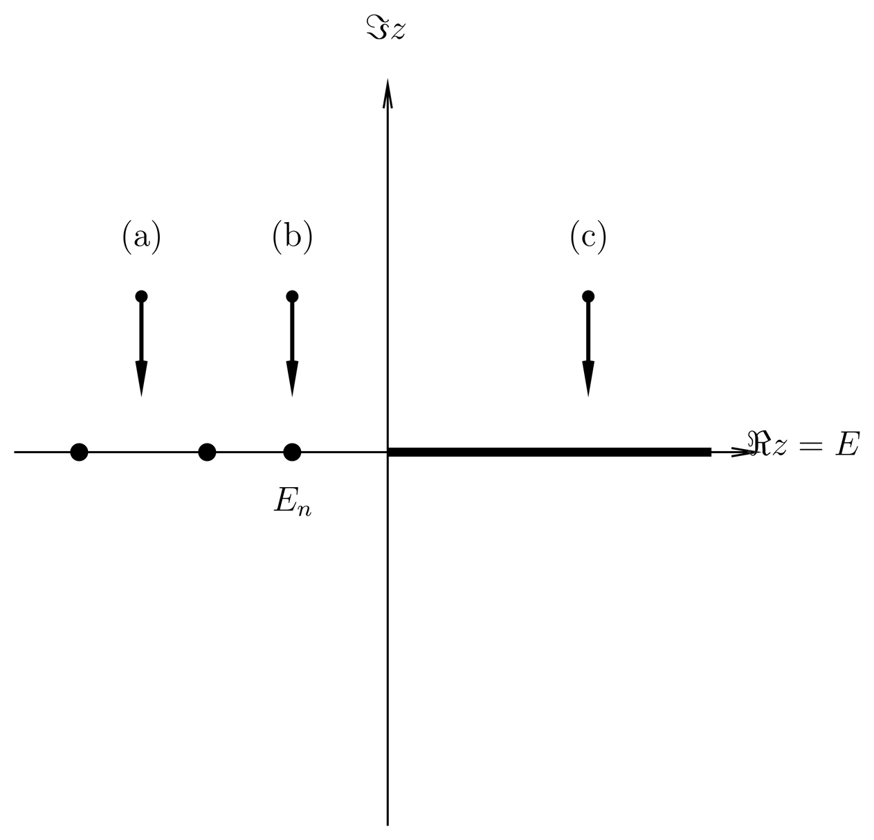
Figure 2:Different cases for the limit in the definition of . The spectrum of consists of a discrete set of negative eigenvalues , plus a continuum of positive eigenvalues (heavy line).
In case (a), is not equal to any of the eigenvalues of , either discrete or continuous. This means that is a negative energy lying in one of the gaps between the discrete, negative eigenvalues . In this case, as none of the denominators in (63) vanish, either in the discrete sum, where any , or in the continuous integral, where the variable of integration is positive while . Thus, the limit is defined, and . The inverse of is meaningful and unique for such real energies.
In case (b), is equal to , one of the discrete, negative eigenvalues of a bound state of the system. In this case, one of the terms in the sum (63) diverges as , in fact, for small the sum is dominated by one term that is proportional to the projection operator onto the eigenspace corresponding to ,
(see Projection Operators). For such energies the Green’s operator does not exist (it diverges).
In case (c), , so as we approach one of the positive eigenvalues of the continuous spectrum of . In this case, none of the denominators in the discrete sum in (63) vanish, but the denominator under the integral does approach zero at , which is part of the range of integration. As it turns out, the limit of the integral as is defined nevertheless. We will not prove this fact, but we will work out an example later (in \secrgreensfuns-18) in which we will see that the -integral is well behaved as , in spite of the singularity in the integrand. Thus, for , is defined. It would be tempting to write simply for this operator, but at positive energies taking the limit is not the same as just setting . In particular, if we just set in (63), then the integral is not defined as it stands due to the singularity in the integrand at . When integrals like this arise some books simply offer a “prescription” of replacing by (whereupon the integral is defined) and then taking the limit. This prescription, as we see, amounts to using the outgoing Green’s function. At positive energies (energies belonging to the continuous spectrum) it is better not to use the notation . Instead, it is better to be more explicit and write .
Now we must prove that , when it is defined (that is, when is not equal to any of the discrete, bound state eigenvalues ), is actually a Green’s operator for the inhomogeneous Schr"odinger equation (43). That is, we must show that it satisfies (48). We do this by using the definition (64),
where in the second equality we add and subtract inside the first factor and in the third equality we use the fact that the inverse of is well defined when . In the final step we use the assumption that is such that is defined, so the limit of is zero.
Since , defined whenever is not equal to one of the discrete eigenvalues of , is a Green’s operator for the operator , the corresponding Green’s function can be used to solve the inhomogeneous Schr"odinger equation (43) for such energies. In the next set of notes we shall show how this is used in scattering theory, but first we must examine another energy-dependent Green’s operator.
The Incoming Energy-Dependent Green’s Operator
The incoming energy-dependent Green’s operator, denoted , is defined basically as the Fourier transform of the incoming time-dependent Green’s operator ,
apart from convergence issues. Compare this to definition (56) for the outgoing Green’s operator. Recall that , so this integral is cut off for positive times, and can be written
The integral can be done, but the antiderivative does not converge at the lower limit , much as was the case with the integral for at the upper limit . In this case we cure the problem by replacing by in the Schr"odinger equation, which causes all solutions to grow as , thereby guaranteeing that any solution that is finite at is zero at (the solutions damp if you go backwards in time). This substitution is equivalent to replacing by in (68), thereby pushing the energy into the lower half of the complex plane and leading to the definition
where now . Compare this to (58); the final answer is the same formula, but it is defined in different parts of the complex energy plane.
Analyzing as we did above with , we find that it is well defined in the entire lower half plane (). To get a Green’s operator defined at physical (real) values of , we define
a limit that exists as long as is not equal to any of the discrete, bound state eigenvalues of . Where the limit does exist, is a legitimate Green’s operator, that is, it satisfies
and so can be used to solve inhomogeneous Schr"odinger equations.
We did not present any situation analogous to the incoming Green’s function in our discussion of water waves in \secrgreensfuns-10. It turns out that in cases (a) and (b), the water wave field corresponding to the incoming Green’s function is the same as that for the outgoing Green’s function (for the same value of ). In particular, the incoming Green’s function also diverges when is equal to one of the eigenfrequencies of a finite lake and . But in case (c), the wave field on the infinite ocean is different in the two cases (incoming and outgoing). Whereas the outgoing wave field consists of waves carrying a steady flux of energy away from the driver out to infinity, the incoming wave field carries energy in the opposite direction. That is, in the limit of zero damping, the water wave field on the infinite ocean corresponding to the incoming Green’s function consists of waves carrying a steady flux of energy inward from infinity, concentrating it in ever smaller regions of space near the driver, which finally absorbs this energy.
It is obvious that it would be very difficult to set up even an approximation to the incoming wave field experimentally, while setting up the outgoing wave field would be easy. Correspondingly, the incoming Green’s function is not used in solving actual scattering problems, but it is useful in studying theoretical aspects of scattering.
The Discontinuity Across the Real Energy Axis
We should not be surprised to find more than one Green’s function or operator, since these are not unique. This is because Green’s functions are themselves solutions of an inhomogeneous wave equation, for example, (45), and are only determined by that equation to within the addition of a solution of the homogeneous equation. Thus the difference between any two Green’s functions is a solution of the homogeneous equation (in our case, it is an eigenfunction of with energy ).
Nevertheless, since we have two specific Green’s operators defined for real energies , it is of interest to compute the difference between them. Let us denote the difference by ,
This limit is easier to understand if we replace by and by , and consider the analogous limit for ordinary numbers (not operators):
The final fraction is a quantity that approaches zero as for all , but it approaches infinity as when . Moreover, regarded as a function of it is a Lorentzian function with area that is independent of ,
and it becomes ever more sharply localized about as . It is, therefore, a representation of the -function,
Thus we can write (73) as
The operator is strange-looking, but it is defined by the methods of A Function of an Observable. In particular, expanding this operator in the eigenbasis of , we have
Let us examine in the three cases considered above. When lies in the gaps between the negative eigenvalues of (case (a)), then the -functions in the sum over discrete states are all zero, since any . Also, the -function under the integral over positive energies vanishes, since and . Thus, for such energies, and and approach the same limit (the operator , which is well defined and unique for such energies). In case (b), when for some , one of the -functions in the sum over discrete states is infinity, and is not defined for such energies (it diverges). In case (c), when , the -functions in the discrete sum all vanish, but the -function under the integral gives a nonzero answer, and we find
Later we will evaluate this final expression explicitly for the case of a free particle.
We see that for positive energies, the two Green’s operators are well defined, but they are not the same operator. This is why notation like is ambiguous for such energies; instead, it is better to be more explicit and to write .
The Green’s Operator as an Analytic Function of Complex Energy
These results show that is the analytic continuation of through the gaps between the discrete, negative eigenvalues of , and that, in a sense, these are the same operator, call it , uniquely defined everywhere in the complex energy plane where , with certain limits as the real axis is approached from above or below. This operator is called the resolvent. It may be expanded in the energy eigenbasis,
It is natural to borrow language from complex variable theory to describe the dependence of on , even though the usual notion of an analytic function applies to a complex-valued function of a complex variable, and we have here an operator-valued function. Without defining what the latter means precisely we just remark that one can always speak of the matrix elements of the resolvent, that is, the Green’s function
which is a complex-valued function of .
From this point of view we see from the expansion (80) that the resolvent is an analytic function of whenever none of the denominators vanish, that is, everywhere in the complex plane where and on the negative real axis between the discrete eigenvalues. The resolvent evidently has poles at the discrete, negative, bound state eigenvalues , whose residues are the projectors onto the corresponding energy eigenspaces. The residues can be picked up from a Cauchy-type contour integral that only samples at values for which it is defined,
where the contour , illustrated in Figure 3, encloses the pole at (and no other).
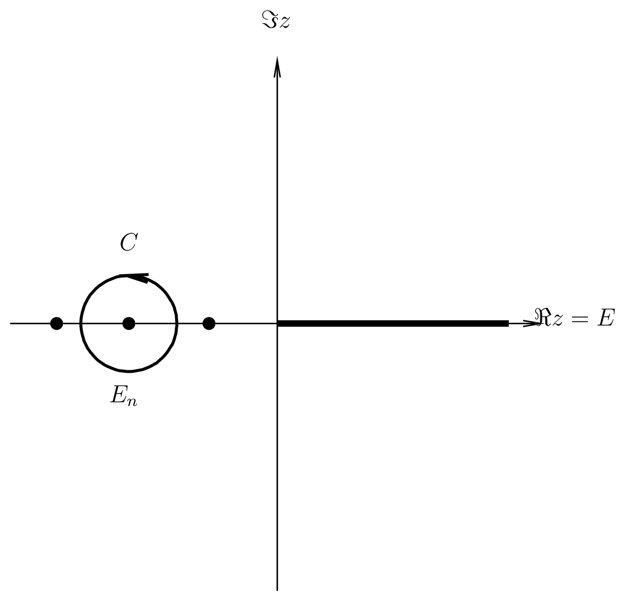
Figure 3:Contour for the integral (82), giving the projector onto the energy eigenspace with eigenvalue .
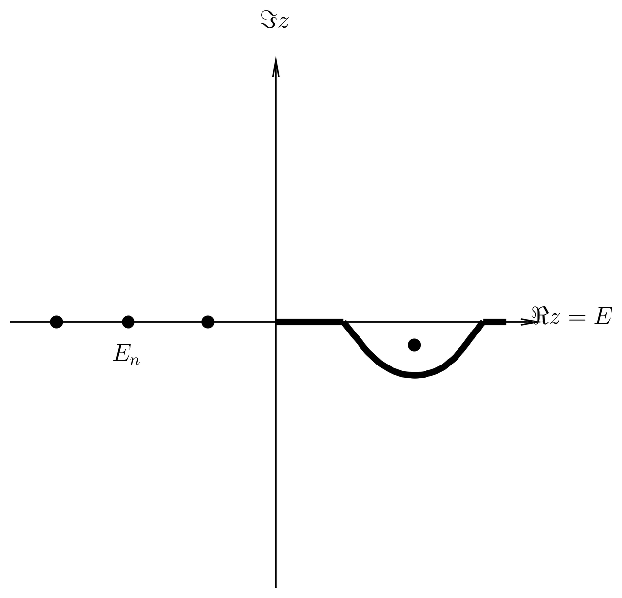
Figure 4:The branch cut at positive energies can be deformed, revealing further singularities of on a second Riemann sheet.
As for the continuous spectrum of on the positive real energy axis, approaches different values as approaches from above or below. This is interpreted by saying that has a branch cut extending from to along the real axis, whose discontinuity is the operator given by (77). on one side of this branch cut can be analytically continued across the branch cut to the other side, but the result is not on the other side, rather it is on a second Riemann sheet that is revealed when we push the branch cut aside. See Figure 4, where is analytically continued from the upper half plane into the lower. When this is done, sometimes further singularities are revealed, which like those on the first (original) Riemann sheet have physical significance. In particular, a pole on the second Riemann sheet in the lower half complex plane represents a resonance of the Hamiltonian , that is, a long-lived state that is actually part of the continuum but which behaves for short times (short compared to the decay time) as if it were a discrete energy eigenstate. We have seen resonances previously in one-dimensional problems (which we analyzed by WKB theory, see Prob. Paragraph), and in the doubly excited states of helium (see The Doubly Excited States). We will encounter them again when we study the decay of excited atomic states by the emission of a photon, in 44. Natural Line Width, Long-Time Behavior and the Lamb Shift.
We see that the singularities of contain coded within themselves all of the physical information we might require about the Hamiltonian : its discrete eigenvalues, the projectors onto the corresponding eigenspaces (from which the bound state eigenfunctions may be extracted), the continuous spectrum, and even the resonances. As we shall see, the resolvent also allows us to compute the scattering amplitude and the (related) -matrix for positive energies. As such, the operator is an object of central importance in quantum mechanics.
This very richness, however, means that finding explicitly is equivalent to (and just as difficult as) solving the original Hamiltonian , and that for most practical problems we will have to resort to perturbation theory or numerical methods to find . We will shortly see some perturbative approaches to finding , and Prob. Paragraph is an example in which the exact Green’s operator can be found analytically.
The Free-Particle Green’s Functions 
As an example, let us compute the outgoing and incoming Green’s functions for a free particle. This case is simple enough that we can do all the calculations explicitly, and it is important also for applications to scattering theory. We denote the free particle Green’s functions (outgoing and incoming) by , with a 0-subscript that means “free particle.” We shall compute these Green’s functions both for and , and use them to illustrate some of the general theory presented above.
To find we use (58) with , deferring the limit until later. We introduce the momentum representation, in which is diagonal, so that
where we use
(84) makes it clear that the Green’s function depends only on the vector difference,
(this is a consequence of the translational invariance of the free-particle Hamiltonian ).
We change variables of integration in (84) by and we write
so that is a complex version of . The parameter is specified in terms of the complex energy by
but we must say which of the two square roots is intended. We treat as small and illustrate the two cases and in Figure 5. When , we take to lie just above the real axis, like in the figure. When , we take to lie just to the right of the imaginary axis, like in the figure. Then as , we define
where
and
Thus, is the usual wave number for positive energies, while is the exponential decay factor for free-particle solutions of negative energy.
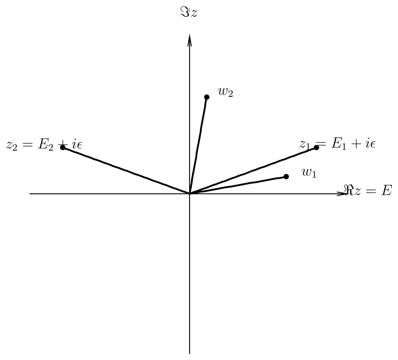
Figure 5:Defining the branch of , the complex version of the wave number , in the case (outgoing Green’s function).
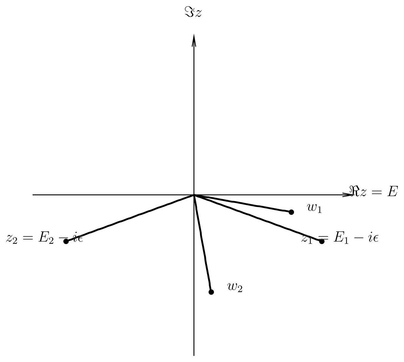
Figure 6:Doing the same for the case (incoming Green’s function).
With these changes of notation we have
This equation makes it clear that the Green’s function actually depends only on the magnitude of , since the integral is invariant if we replace by , where is any rotation matrix. This is due to the rotational invariance of the Hamiltonian . Therefore without loss of generality we can place on the -axis, so that , where is the usual spherical angle in -space and where
Then carrying out the angular integrations we have
As for the term with , we substitute and drop the prime, which makes the integrand the same as the first term, but with range of integration to 0. Thus the two terms together are
This final integral can be evaluated by Cauchy’s residue theorem. The integrand decays exponentially in the upper half -plane, so we can close the contour of integration with a semicircle at infinity, which then picks up the pole at . Notice that it is essential that be off the real axis (that is, ) for this to work. The result is
where it is understood that and that lies in the first quadrant.
We may treat the incoming Green’s function similarly, where now . Now lies in the lower half plane and , defined by
can be taken to lie in the fourth quadrant, as illustrated in Figure 6. Now in the limit we have
Evaluating the integral in this case we find
Finally we take the limit , using either (89) or (98) for the outgoing and incoming cases, respectively. The results can be summarized by
One point to notice is that this limit exists. This is an example of the integral in (63) when , showing that the limit exists when , in spite of the fact that the integrand diverges at one point.
(100) gives the Green’s functions explicitly for a free particle. Each satisfies the inhomogeneous Schr"odinger equation (45), which in the case of a free particle is
so is a free particle solution of energy at all spatial points except , where and is singular. For , the free particle solution in the region consists of spherical waves either radiating outward (for ) or inward (for ). (The waves are seen to radiate one direction or another when we attach the time dependence .)
Discontinuity for the Free Particle
As predicted in \secrgreensfuns-16, the Green’s functions are analytic continuations of one another across the negative real energy axis, where of course there are no poles for discrete states because this is the case of a free particle. That is, for . As for the positive energy axis, there is a discontinuity given by
According to (77), this final result should be the matrix element,
We leave it as an exercise to show that this is true. (One can compute the matrix element by switching to a momentum representation, as we did in (84) for the Green’s function.)