07. The WKB Method

Introduction¶

The WKB method is important both as a practical means of approximating solutions to the Schr"odinger equation and as a conceptual framework for understanding the classical limit of quantum mechanics. The initials stand for Wentzel, Kramers and Brillouin, who first applied the method to the Schr"odinger equation in the 1920’s. The WKB approximation is also called the semiclassical or quasiclassical approximation. The basic idea behind the method can be applied to any kind of wave (in optics, acoustics, etc): it is to expand the solution of the wave equation in the ratio of the wavelength to the scale length of the environment in which the wave propagates, when that ratio is small. In quantum mechanics, this is equivalent to treating $\hbar$ formally as a small parameter. The method itself antedates quantum mechanics by many years, and was used by Liouville and Green in the early nineteenth century.

Planck’s constant $\hbar$ has dimensions of action, so its value depends on the units chosen, and it does not make sense to say that $\hbar$ is “small.” However, typical mechanical problems have quantities with dimensions of action that appear in them, for example, an angular momentum, a linear momentum times a distance, etc., and if $\hbar$ is small in comparison to these then it makes sense to treat $\hbar$ formally as a small parameter. This would normally be the case for macroscopic systems, which are well described by classical mechanics. Thus the classical limit can be thought of as one in which $\hbar$ is small in comparison to typical actions of the system.

It is obvious that there must be some subtlety in the classical limit of quantum mechanics, since the physical interpretations of the two theories are so different. For example, quantum mechanics makes physical predictions that are fundamentally statistical, while statistics only enters into classical mechanics if there is a lack of complete information about initial conditions. Moreover there are quantum phenomena, such as interference and tunneling, that have no classical analog. We will see as we proceed how WKB theory represents these characteristic features of quantum mechanics around a framework constructed out of classical mechanics.

The WKB Ansatz¶

As mentioned the WKB method can be applied to any wave system in which the wavelength is small compared to typical scale lengths of the system, so we have a wide choice of systems with which to illustrate the method. We will begin with the time-independent Schr"odnger equation in three dimensions for a particle moving in a potential $V(\xvec)$ , because the multidimensional case makes certain aspects of the classical limit more vivid. Another interesting case would be the time-dependent Schr"odinger equation, for which see Other Types of Problems. This offers an intuitive presentation of the WKB ansatz, which is a description of how the wave function depends on $\hbar$ , and the beginnings of the classical picture associated with it.

The time-independent Schr"odinger equation that we will use is

-{\hbar^2\over 2m} \del^2 \psi(\xvec) +V(\xvec)\psi(\xvec) = E \psi(\xvec),

(1)

where $E$ is an energy eigenvalue. The quantum Hamiltonian is

H={\pvec^2\over 2m}+V(\xvec),

(2)

a formula that also serves as the classical Hamiltonian, of course with different interpretation of the symbols $\xvec$ and $\pvec$ .

In the special case that the potential is constant, $V=V_0=const.$ , solutions exist in the form of plane waves,

\psi(\xvec) = A e^{iS(\xvec)/\hbar},

(3)

where $A$ is the constant amplitude, and where

S=\pvec\cdot\xvec.

(4)

The vector $\pvec$ is a momentum, and in fact the wave function (3) is an eigenfunction of momentum as well as energy, with eigenvalues related by

E = {\pvec^2 \over 2m} + V_0.

(5)

We assume that $E\ge V_0$ , so that $\pvec$ is real.

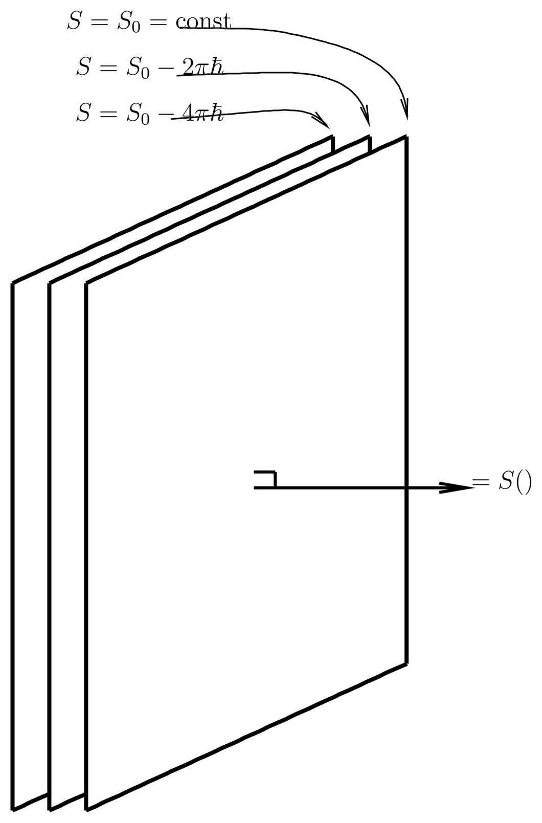
Plane waves are so called because the surfaces of constant phase are planes. The momentum eigenvalue is \pvec=\del S, where S/\hbar is the phase. — Figure 1:Plane waves are so called because the surfaces of constant phase are planes. The momentum eigenvalue is $\pvec=\del S$ , where $S/\hbar$ is the phase.

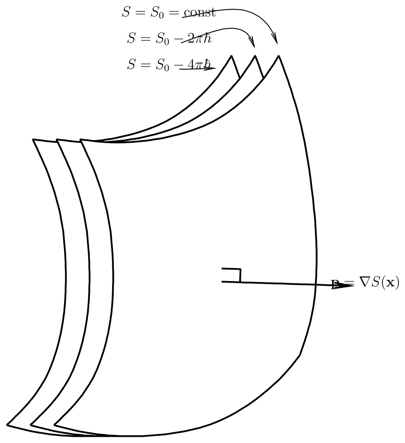
In a slowly varying potential, the wave fronts are surfaces that curve with the same scale length as the potential. The vector \pvec=\del S is a “local momentum,” that is, a function of position. — Figure 2:In a slowly varying potential, the wave fronts are surfaces that curve with the same scale length as the potential. The vector $\pvec=\del S$ is a “local momentum,” that is, a function of position.

The wave (3) is called a plane wave because the wave fronts, that is, the surfaces of constant phase, are planes. These are sketched in Figure 1. The momentum $\pvec = \del S$ is orthogonal to the wave fronts; it is a constant (independent of position). Two wave successive wave fronts with a phase difference of $2\pi$ , that is, with $\Delta S = 2\pi\hbar$ , are separated by the wavelength $\lambda$ , which is related to the momentum by the de~Broglie formula,

\lambda = {2\pi\hbar \over |\del S|} ={2\pi\hbar \over |\pvec|}.

(6)

Now let us consider the case of a slowly varying potential $V$ . Let $L$ be some characteristic scale length of the potential. When we say that $V$ is slowly varying, we mean that $V$ does not change much on the scale of a wavelength, that is,

\lambda \ll L.

(7)

Then it is plausible that the wave fronts, that is, the surfaces of constant phase of the solution $\psi(\xvec)$ of the Schr"odinger equation (1), will be curved surfaces such as illustrated in Figure 2, and that these surfaces will deviate significantly from a plane on the same scale length $L$ as the potential. We can still write the phase of the wave as $S(\xvec)/\hbar$ , but the function $S$ no longer has the plane wave form (4). As for the amplitude $A$ of the wave, it is constant in a constant potential, so it is reasonable to guess that in a slowly varying potential it is also slowly varying, that is, that it has the same scale length $L$ as the potential. We still write the wave function as

\psi(\xvec) = A(\xvec) e^{iS(\xvec)/\hbar},

(8)

but now $A$ and $S$ are functions of $\xvec$ to be determined.

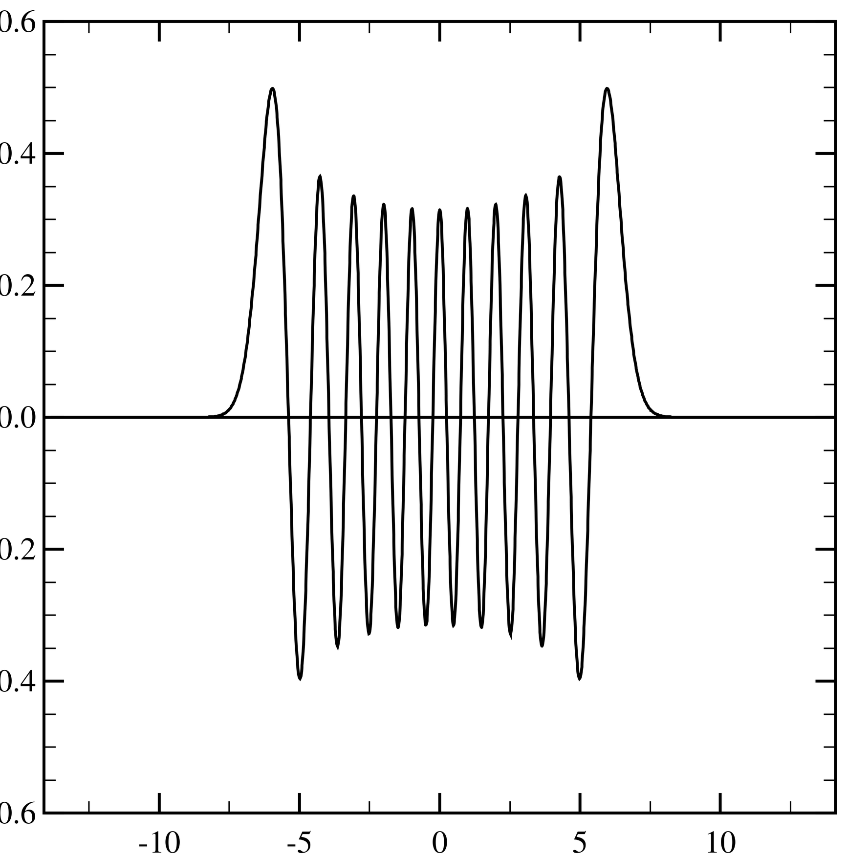
Normalized harmonic oscillator eigenfunction for n=20. Distance x is measured in units of (\hbar/m\omega)^{1/2}. — Figure 3:Normalized harmonic oscillator eigenfunction for $n=20$ . Distance $x$ is measured in units of $(\hbar/m\omega)^{1/2}$ .

Same as , except n=40. — Figure 4:Same as Figure 3, except $n=40$ .

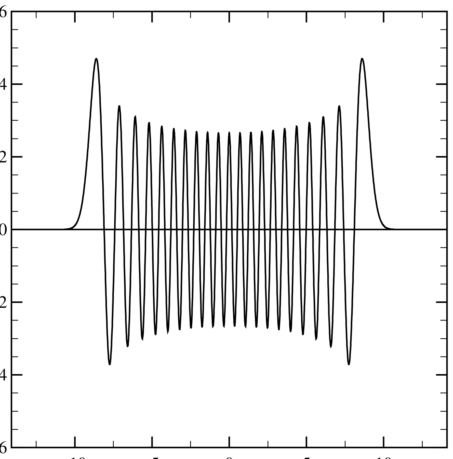
Some exactly solvable one-dimensional problems reinforce our confidence in the validity of (8) and the assumptions surrounding it. See, for example, the one-dimensional eigenfunctions of the harmonic oscillator illustrated in Figs.~Figure 3 and Figure 4. The wave function is largely concentrated between the classical turning points for the given energy $E$ , namely, $\pm (2E/m\omega^2)^{1/2}$ . We can take $L$ as the distance between these turning points. The wave function $\psi(x)$ looks like a cosine wave (a sum of two terms of the form (8)) with a slowly varying amplitude and wave length.

Returning to the three-dimensional case, it is clear from Figure 2 that the solution $\psi(\xvec)$ looks like a plane wave if we examine it in a region of space small compared to $L$ . Let $\xvec_0$ be a fixed point of space, and let $\xvec = \xvec_0 + \xivec$ , where $|\xivec| \ll L$ . Then when we expand the wave function (8) about $\xvec_0$ , we can simply evaluate the amplitude $A$ at $\xvec_0$ , since it does not change much on the scale of $\xivec$ , but we must include the first correction term in the phase. Thus we have

\psi(\xvec_0+\xivec) \approx A(\xvec_0)e^{iS(\xvec_0)/\hbar} e^{i\xivec \cdot \del S/\hbar},

(9)

where the first two factors constitute a constant amplitude and phase, and the third shows that $\psi$ has locally the form of a plane wave with momentum

\pvec=\pvec(\xvec)=\del S(\xvec).

(10)

Unlike the case of a plane wave, $\pvec$ is now a function of position, so it is not constant and $\psi(\xvec)$ is no longer an eigenfunction of momentum. (The wave function $\psi(\xvec)$ is still an eigenfunction of energy, however, with energy $E$ .) The local momentum $\pvec(\xvec)$ is orthogonal to the wave fronts, as illustrated in Figure 2. Since displacement by the wave length $\lambda$ in a direction orthogonal to the wave fronts must result in a phase advance of $2\pi$ , the de~Broglie relation (6) still holds, but now $\lambda$ is also a function of position. Notice that the assumption (7) can be stated in another form,

{\hbar \over |\pvec| L } \ll 1,

(11)

showing the dimensionless ratio of a mechanical action to $\hbar$ .

The momentum field (10) gives us the beginning of a classical interpretation of the solution (8) of the Schr"odinger equation. That is, we imagine that the region of space occupied by the wave (8) is also occupied by a swarm of classical particles, such that the particle at position $\xvec$ has momentum $\pvec(\xvec)=\del S(\xvec)$ . This swarm defines in effect a classical ensemble out of which the probabilistic features of quantum mechanics will be represented. The momentum field $\pvec(\xvec)$ satisfies

\del \cross \pvec(\xvec) = 0,

(12)

and

S(\xvec) = S(\xvec_0) + \int_{\xvec_0}^{\xvec} p(\xvec') \cdot d\xvec',

(13)

where in the latter integral $\xvec$ and $\xvec_0$ are any two points and the path of integration is any path between them (we ignore topological complications in the application of Stokes’ theorem). Integrals of the form (13) are well known in classical mechanics, where the function $S$ is called Hamilton’s principal function. It is also called simply the action, and it does have dimensions of action, but several different quantities in classical mechanics are called the action and one should be aware of which is meant when using this term. It was because of the interpretation of the function $S$ as the classical action that we split off a factor of $\hbar$ in the phase of the quantum wave function in (3) and (8).

The notion of the momentum field $\pvec(\xvec)$ leads to further questions. Obviously the momentum of a classical particle moving in the potential $V(\xvec)$ would change as the particle moves on its orbit. Suppose at $t=0$ we consider the particle at position $\xvec_0$ which has momentum $\pvec_0=\pvec(\xvec_0)$ . Then $(\xvec_0,\pvec_0)$ forms a complete set of initial conditions for a classical orbit. If we follow this classical orbit for some amount of time, the particle moves to a new position $\xvec_1$ . Is the momentum of the particle following this orbit the same as the value of the momentum field $\pvec(\xvec)$ , evaluated at $\xvec=\xvec_1$ ? The answer is yes, at least within the framework of the WKB approximation.

The momentum field $\pvec(\xvec)$ can be associated with a velocity field

\vvec(\xvec)={\pvec(\xvec)\over m},

(14)

and an energy field

E(\xvec) = {\pvec(\xvec)^2\over 2m}+V(\xvec),

(15)

so that the classical particle at $\xvec$ has momentum $\pvec(\xvec)$ , velocity $\vvec(\xvec)$ and energy $E(\xvec)$ . All of these follow from the phase $S(\xvec)$ of the quantum wave function. If that wave function is a solution of the Schr"odinger equation (1), then what is the relation between the energy field $E(\xvec)$ and the energy eigenvalue $E$ ? The answer is that they are equal, that is, the energy field $E(\xvec)$ that we have defined in (15) is actually a constant (independent of $\xvec$ ).

It turns out that the ensemble of classical particles also has a density, which perhaps not surprisingly is given by

\rho(\xvec)=|\psi(\xvec)|^2 = A(\xvec)^2,

(16)

where we use the WKB ansatz (8). That is, the density of particles in the classical ensemble is the same as the quantum probability density (at least this is true in the WKB approximation). More precisely, for bound energy eigenfunctions, which are normalizable, $\rho(\xvec)$ is the probability density; if the eigenfunction is a part of the continuous spectrum then $\rho(\xvec)$ is not normalizable, but it can still be interpreted in the WKB approximation as a density of classical particles associated with the wave.

Given that the particle at position $\xvec$ has velocity $\vvec$ , the motion of the particles under the classical equations of motion gives rise to a particle current,

\Jvec(\xvec)=\rho(\xvec)\vvec(\xvec),

(17)

which is similar to the mass current in a fluid. This current becomes known once the amplitude $A(\xvec)$ and phase $S(\xvec)$ of the quantum wave function are known. As it turns out, it is a consequence of the Schr"odinger equation (1) that this current is divergence-free,

\del\cdot\Jvec(\xvec)=0,

(18)

at least in the WKB approximation. This means that as the classical particles of the ensemble follow their orbits according to the classical equations of motion, the number of particles entering some volume of space equals the number leaving, so that the density $\rho(\xvec)$ remains constant.

This concludes an overview of some of the features of the classical picture associated with the WKB approximation to the solution of the time-dependent Schr"odinger equation (1). We will now develop this solution more carefully.

Equations for $S$ and $A$ ¶

To obtain equations for $S$ and $A$ we can take the WKB ansatz (8) and substitute it into the Schr"odinger equation (1), neglecting higher order terms in $\hbar$ . A more systematic and cleaner way of doing this, and one that in principle allows us to compute all the higher order corrections in $\hbar$ , is the following.

First we bring the amplitude up into the exponent by writing the WKB ansatz as

\psi(\xvec) = \exp\Bigl\{ {i\over\hbar} [S(\xvec) -i\hbar\ln A(\xvec)] \Bigr\}.

(19)

From this we see that the amplitude (or, rather, $-i\ln A$ ) is in a sense the $O(\hbar)$ correction to the action $S$ . We extend this expansion to all orders, writing

\psi(\xvec) = \exp\Bigl[ {i\over\hbar} W(\xvec) \Bigr],

(20)

where

W(\xvec) = W_0(\xvec) + \hbar W_1(\xvec) + \hbar^2 W_2(\xvec) + \ldots,

(21)

and where

W_0(\xvec) = S(\xvec), \qquad W_1(\xvec) = -i \ln A(\xvec).

(22)

With this approach we are exploring the classical limit of quantum mechanics by expanding the logarithm of the wave function in powers of $\hbar$ , in which the leading term is $O(1/\hbar)$ . It will not do to expand the wave function itself in powers of $\hbar$ , since $\psi$ simply oscillates ever more rapidly as $\hbar\to0$ , and does not approach a limit.

The WKB ansatz (8) looks like just the decomposition of the complex wave function $\psi$ into its amplitude and phase, in the sense of complex numbers, with the additional information that the phase behaves as $1/\hbar$ as $\hbar\to0$ . It would be that, and the WKB ansatz would be exact, if we required that $A$ and $S$ be real. But in that interpretation both $A$ and $S$ would have a dependence on $\hbar$ . By expanding $W$ in powers of $\hbar$ as we have done in (21), we have in effect redefined $S$ and $A$ in terms of the zeroth and first order terms of $W$ , so that now $S$ and $A$ have no $\hbar$ dependence. This means that there are now higher order corrections ( $W_2$ , etc), so that the WKB anstaz (8) is only an approximation. Also, there is no longer any requirement that $S$ and $A$ be real. Indeed, as we shall see in one-dimensional problems, $S$ takes on complex values in the classically forbidden region.

We now substitute (20) into the Schr"odinger equation (1), and express the latter in terms of $W$ instead of $\psi$ . After a little algebra, we find

{1\over 2m} (\del W)^2 -{i\hbar\over 2m} \del^2 W + V =E.

(23)

No approximations have been made yet, and this is exactly equivalent to the Schr"odinger equation (1), although the shift from $\psi$ to its logarithm has made the Schr"odinger equation nonlinear. Next we expand $W$ as in (21), substitute into (23), and collect terms order by order. At order $\hbar^0$ , we find

{1\over 2m} (\del W_0)^2 + V(\xvec) = E,

(24)

{1\over 2m} (\del S)^2 + V(\xvec) = E.

(25)

This is the well known Hamilton-Jacobi equation of classical mechanics. See (137). Notice that with $\pvec(\xvec)=\del S$ the Hamilton-Jacobi equation confirms the remark made about (15), that the energy field $E(\xvec)$ is constant and equal to the energy eigenvalue. All the particles of the classical ensemble associated with the energy eigenfunction (20) have the same energy, which is the energy eigenvalue of the quantum problem.

At order $\hbar^1$ , we find

{1\over m} \del W_0 \cdot \del W_1 - {i\over 2m} \del^2 W_0 =0,

(26)

or by (22),

{1\over m}\del S \cdot \del \ln A + {1\over 2m} \del^2 S=0.

(27)

We multiply this by $2A^2$ and use $\vvec(\xvec)=\pvec(\xvec)/m=\del S/m$ , which gives

\vvec\cdot(2A\del A) + A^2 \del\cdot\vvec=0,

(28)

\del\cdot (A^2 \vvec) = 0.

(29)

We call this equation (in its various forms) the amplitude transport equation.

If the amplitude $A$ and action $S$ are real, as they are in classically allowed regions, then the amplitude transport equation is the WKB approximation to the continuity equation (55) for the probability density and current, which of course is exact. We see this by neglecting terms $W_2$ etc.{} in the expansion (21), so that

\rho(\xvec)=|\psi(\xvec)|^2 \approx A(\xvec)^2,

(30)

and

\Jvec(\xvec)=\Re \psi^\cc \Bigl(-{i\hbar\del\over m}\Bigr)\psi \approx A(\xvec)^2\vvec.

(31)

With these substitutions, the amplitude transport equation becomes $\del\cdot\Jvec=0$ . In comparison to the continuity equation (55), the term $\partial\rho/\partial t=0$ , since $\rho$ is independent of time.

Historical and Other Comments on the Hamilton-Jacobi Equation¶

A version of the Hamilton-Jacobi equation first appeared in Hamilton’s researches in the 1830’s into variational formulations of mechanics and their relation to optics. Hamilton discovered the form of the classical equations of motion that now bears his name, and he realized that their complete solution was equivalent to solving a certain partial differential equation, (39). These ideas were generalized by Jacobi a few years later, who developed methods for solving (32), what we now call the time-independent Hamilton-Jacobi equation. Jacobi used these methods to solve some nontrivial problems in classical mechanics.

Renewed interest in the Hamilton-Jacobi equation arose in the period of the old quantum theory (1900-1925), after Sommerfeld’s and Wilson’s analysis of Bohr’s quantization condition, which is expressed in terms of action integrals like (13). The old quantum theory was a collection of rules that were incomplete, logically unclear, and of limited applicability, but which gave excellent agreement with experiment in a number of important cases such as the specific heat of solids and the spectrum of hydrogen, including its fine structure. As a result, the period 1911-1925 saw a heightened interest in the formal structure of classical mechanics, in the hope that it would elucidate the difficulties of the old quantum theory. These efforts were summarized in Born’s book The Mechanics of the Atom, published just about the time that Heisenberg’s and Schr"odinger’s (modern) quantum theory emerged. After this, interest in classical mechanics, at least in physics circles, fell to almost zero.

In more recent times, since the advent of computers and the discovery of chaos, classical mechanics has enjoyed another revival, partly stimulated also by developments in mathematics such as the KAM (Kolmogorov-Arnold-Moser) theorem. It is now recognized that the Hamilton-Jacobi equation has no global solutions in the case of chaotic motion, and that this has an impact on the morphology and other features of the quantum wave function.

In the language of classical mechanics, the solution $S$ of the Hamilton-Jacobi equation is the generator of the canonical transformation that trivializes the classical equations of motion. The existence of this transformation requires that the system have a sufficient number of commuting constants of motion (the classical analog of a complete set of commuting observables). The constants of motion are conveniently expressed as functions of the actions, themselves constants of motion that generate periodic (and commuting) flows in phase space. The variables canonically conjugate to the actions are certain angles. Such matters are discussed in advanced courses in classical mechanics.

Because of problems with chaos and other issues, the Hamilton-Jacobi equation and the other equations of WKB theory are harder to solve in the multidimensional case, so the most common applications of WKB theory are in one dimension. We now turn to that case.

One-Dimensional WKB Problems¶

We consider now the one-dimensional Schr"odinger equation,

-{\hbar^2\over 2m} \psi''(x) + V(x)\psi(x) = E\psi(x),

(42)

in which we use the one-dimensional WKB ansatz,

\psi(x) = A(x) e^{iS(x)/\hbar}.

(43)

The Hamilton-Jacobi equation is the one-dimensional version of (25),

{1\over 2m}\Bigl( \dod{S}{x} \Bigr)^2 + V(x) =E,

(44)

and the amplitude transport equation is the one-dimensional version of (29),

\dod{}{x} \Bigl(A^2 \dod{S}{x} \Bigr)=0.

(45)

We solve the Hamilton-Jacobi equation (44) algebraically for $dS/dx$ , obtaining

\dod{S}{x} = p(x) = \pm \sqrt{2m[E-V(x)]}.

(46)

The ± sign means that there are actually two WKB solutions, with actions that differ by a sign. The general solution is a linear combination of the two solutions. Integrating (46), we have

S(x) = \int_{x_0}^x p(x') \, dx'.

(47)

Changing the lower limit of integration merely adds a constant to $S$ , which by (43) just changes the overall phase of the wave function. We will worry about phases later, and for now we set $x_0$ to anything convenient.

The amplitude transport equation (45) is also easily solved. We find

A(x) = {\\textconst \over \sqrt{p(x)}},

(48)

where as we see by (43) the constant of integration just establishes the normalization and phase of the wave function. For now we set this constant to anything convenient.

To proceed it is convenient to get rid of the ± sign in (46) by committing to a definite branch of the square root function. How we do this depends on whether $E>V(x)$ (a classically allowed region, where the kinetic energy is positive and the momentum real) or $E<V(x)$ (a classically forbidden region, where the kinetic energy is negative and the momentum imaginary). We will adopt the following definitions,

\begin{aligned} p(x) = \begin{cases} \sqrt{2m[E-V(x)]}, & E> V(x), \\ i\sqrt{2m[V(x)-E]}, & E < V(x). \\\end{cases} \end{aligned}

(49)

Then we will define $S(x)$ by (47), and say that the solutions of the Hamilton-Jacobi equation (44) are $S(x)$ and $-S(x)$ , with associated momentum functions $p(x)$ and $-p(x)$ . The momentum is purely imaginary in the classically forbidden region.

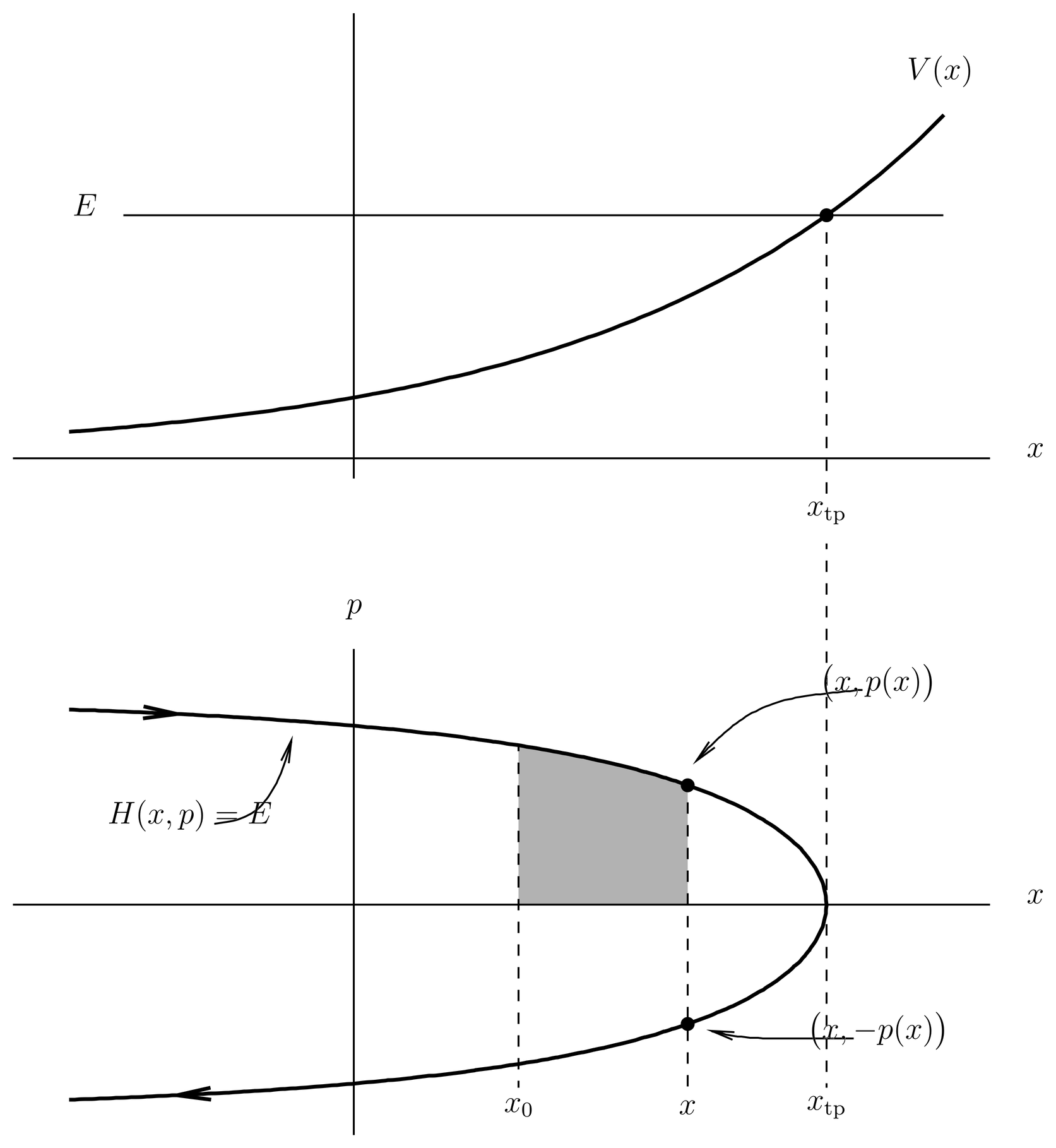
Illustration of functions p(x) and S(x) in classically allowed region. — Figure 5:Illustration of functions $p(x)$ and $S(x)$ in classically allowed region.

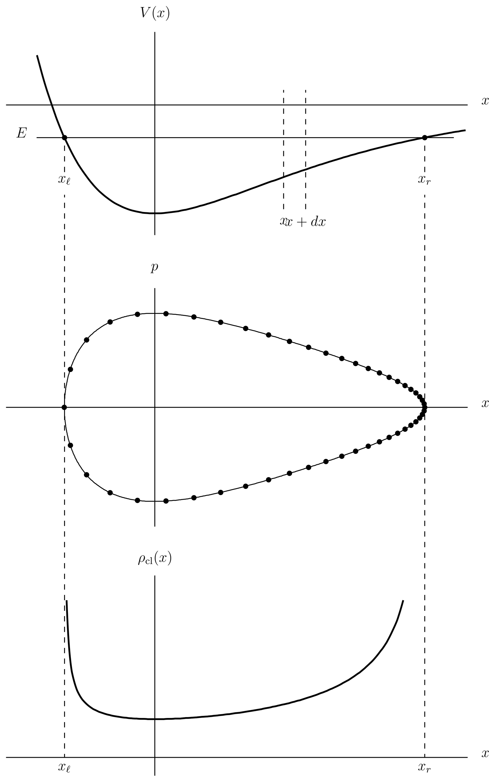
Meaning of classical probability density \rho(x) for a one-dimensional oscillator (the Morse oscillator). — Figure 6:Meaning of classical probability density $\rho(x)$ for a one-dimensional oscillator (the Morse oscillator).

The classical meaning of the functions $p(x)$ and $A(x)$ may be seen in Figure 5, which illustrates a portion of the $x$ -axis in which there is a classical turning point $x_tp$ (a point where $E=V(x)$ ), with the classically allowed region to the left and the classically forbidden region to the right (upper part of figure). The energy $E$ is the eigenvalue of the Schr"odinger equation (42). The lower part of the figure is a phase space plot, showing the classical orbit of energy $E$ . The orbit is also the contour line of the classical Hamiltonian, $H(x,p)=E$ , because the classical motion conserves energy and therefore traces out this line. A given $x$ value in the classically allowed region corresponds to two momentum values, $\pm p(x)$ , where the vertical line of constant $x$ intersects the orbit, representing the particle passing $x$ going one direction, and then passing it again going back. These are the two momentum branches corresponding to a given $x$ value. Thus, the upper branch (the upper part of the orbit in phase space) is the graph of the function $p=p(x)$ . By (47), the action $S(x)$ with lower limit $x_0$ is the area between the $x$ -axis and the upper part of the orbit and between the limits $x_0$ and $x$ , as in the shaded part of the figure.

We spoke previously of a swarm or ensemble of classical particles that represents the WKB wave, such that the momentum of the particle at position $\xvec$ is $\pvec(\xvec)$ (in three dimensions). From Figure 5, we see that in the one-dimensional case there are really two swarms, one with particles going to the right and one with them going to the left. If the positions and momenta of these particles are plotted in phase space, then they lie on the line $H=E$ , that is, they all have the same classical energy. This, in fact, is the meaning of the Hamilton-Jacobi equation (44).

The amplitude solution (48) also has a classical interpretation. As explained in Equations for $S$ and $A$ , $A(x)^2$ is the same as the quantum probability density $\rho(x)=|\psi(x)|^2$ in the WKB approximation (neglecting $O(\hbar^2)$ and higher terms in the expansion (21)), and it has an interpretation in terms of the density of the ensemble or swarm of classical particles. In the one-dimensional case, this classical density can be understood from another standpoint, which we now discuss. The density in question is only normalizable in the case of an oscillator, so we consider that case, and refer to Figure 6.

The top of the figure is the potential energy curve for the Morse oscillator, which is often used to model the stretching of molecular bonds. The potential rises rapidly to the left, corresponding to the strong repulsion of atoms that are brought close together, and gradually to the right, representing the attractive force between atoms as they are pulled apart, a force that dies off slowly as the distance increases. In the middle is a potential well, in which the oscillations represent molecular vibrations. We use the Morse potential here because it is a strongly nonlinear oscillator that presents features not present in the harmonic oscillator.

The classical particle oscillates between the left and right turning points $x_\ell$ and $x_r$ with a period $T$ . In each period, it passes through a small interval $[x,x+dx]$ twice, once going to the right and once to the left. We define a classical probability density $\rho_cl(x)$ by requiring the probability of the particle to lie in the interval $[x,x+dx]$ to be the fraction of the total period $T$ that the particle spends in this interval. That is, we define

\rho_cl(x) \, dx = {2 \over T} \, dt,

(50)

where $dt$ is the time it takes to pass through the interval once. Thus we have

\rho_cl(x) = {2 \over T} {1 \over v(x)} ={2m\over T}{1\over p(x)}.

(51)

According to (48), this probability density is equal to $A(x)^2$ , to within a constant. The function $\rho_cl(x)$ is plotted in the lower part of Figure 6. It is smallest where the classical particle is moving most rapidly, and conversely.

The density $\rho_cl(x)$ diverges at the turning points, where the velocity goes to zero. One can show that $\rho_cl(x)$ goes like $d^{-1/2}$ when $d$ , the distance from a turning point, is small. Then, since $A(x)$ goes like the square root of $\rho_cl(x)$ , it goes like $d^{-1/4}$ and also diverges near the turning point. Thus, the nominal prediction of WKB theory is that the wave function should diverge at turning points. The exact wave function does not actually diverge there, as can be seen from exact solutions such as those in Figs.~Figure 3 and Figure 4, but it does become large there. In effect, the classical singularity is smoothed out by the uncertainty principle, which also causes some of the wave function to spill over into the classically forbidden region. We shall discuss the behavior of the wave function near turning points more carefully below.

According to (50), the swarm or ensemble of particles representing the WKB wave can be thought of as a large number of particles uniformly distributed in time around the orbit. These are illustrated by the dots placed at equal time intervals along the phase space orbit in the center diagram in Figure 6.

By its construction, $\rho_cl(x)$ is normalized to unity. In the case of a scattering problem, the motion is not periodic and $T \to \infty$ , so the density of classical particles cannot be normalized. It is still meaningful, however, to think of particles uniformly distributed along the orbit in time, in which case we have a particle density $\rho_cl(x)$ that is proportional to $1/p(x)$ , as in the case of an oscillator. It is not surprising that $\rho_cl$ cannot be normalized in this case, since the quantum wave function cannot be normalized, either.

Classically Allowed Region to the Left¶

Let us now examine the case in which we have a classically allowed region to the left of a turning point, with a classically forbidden region on the right, as illustrated in Figure 7. The turning point is denoted $x_r$ (since it is to the right of the classically allowed region). We are only sketching part of the $x$ -axis in this diagram, and we make no assumptions about what the potential does to the left or the right of the diagram. For example, to the left it may rise again, creating a potential well, or just asymptote to zero, making a scattering problem. Or, to the right, it may go down again, creating a barrier the particle can tunnel through.

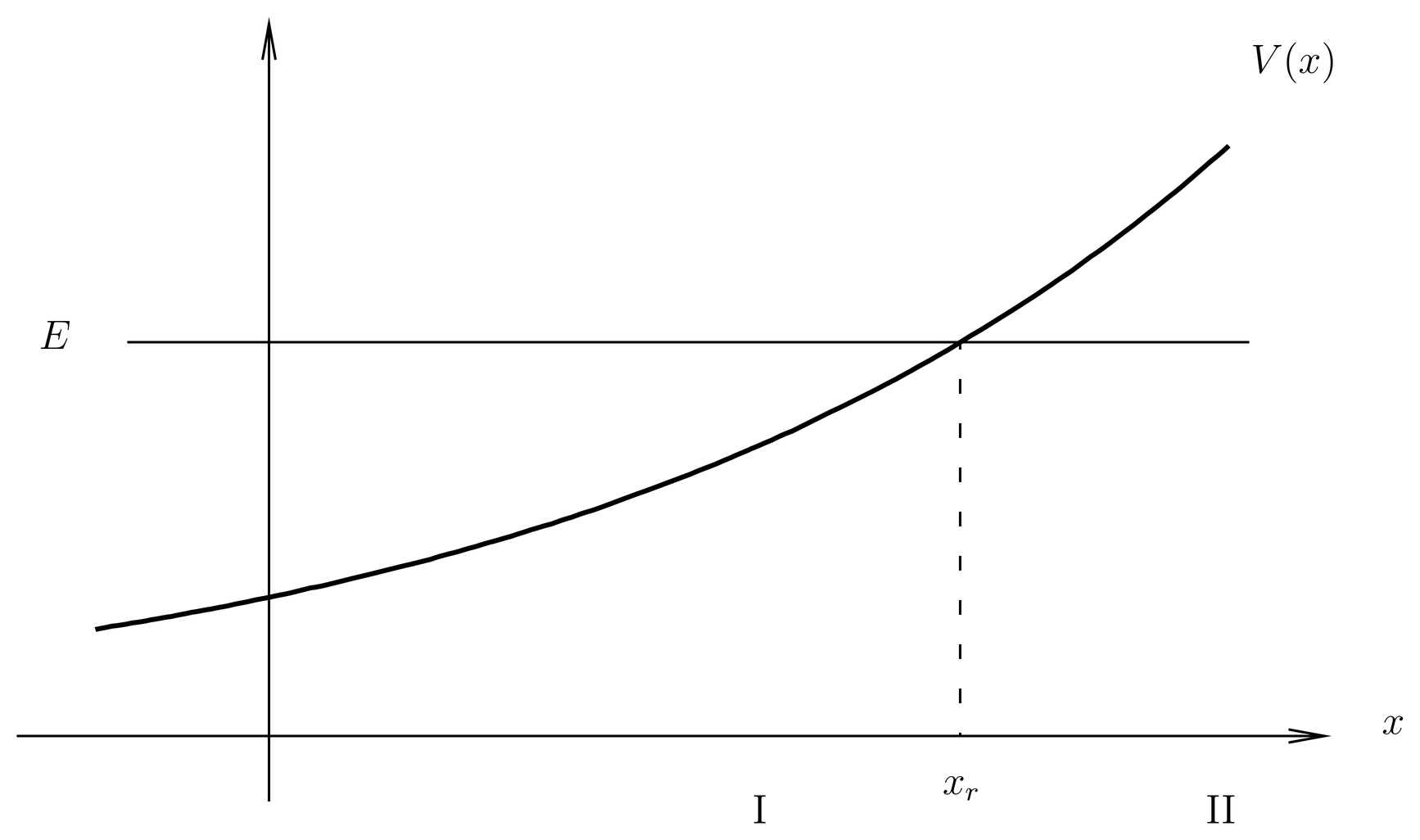
A 1-dimensional potential V(x) rising to the right. Point x_r is a classical turning point. — Figure 7:A 1-dimensional potential $V(x)$ rising to the right. Point $x_r$ is a classical turning point.

First we treat region I, the classically allowed region, where $x<x_r$ and $E>V(x)$ . Here $p(x)$ is real and positive as defined by (49). In this region we define $S$ by

S(x) = \int_{x_r}^x p(x')\, dx',

(52)

which is the same as (47) except that now we are agreeing to measure the action from the turning point $x_r$ . This is merely a matter of convenience, but it means that $S(x)$ is real and negative in region I, and increasing to the right (since $dS/dx = p(x)>0$ ). Taking $S(x)$ and $-S(x)$ as the two solutions of the Hamilton-Jacobi equation, the WKB solution is a general linear combination of two waves,

\psi_I(x) = c_r { e^{iS(x)/\hbar + i\pi/4} \over \sqrt{p(x)}} + c_\ell { e^{-iS(x)/\hbar -i\pi/4} \over \sqrt{p(x)}},

(53)

where $c_r$ and $c_\ell$ are two generally complex constants and where we have introduced phase shifts of $\pm \pi/4$ in the two terms for later convenience. Properly speaking, we should have used $-p(x)$ in the denominator of the second term, but we have absorbed the factor of $\sqrt{-1} = i$ into the second constant. The first term is a wave traveling to the right (since $dS/dx>0$ ), and the second, a wave traveling to the left; this is the meaning of the subscripts on the constants $c_r$ and $c_\ell$ . The general solution is a linear combination of such waves.

Next we treat region~II, the classically forbidden region, where $x>x_r$ and $E<V(x)$ . Here $p(x)$ is purely imaginary, as given by (49). In order to work with real quantities, we define

K(x) = \int_{x_r}^x |p(x')| \,dx' = \int_{x_r}^x \sqrt{2m[V(x')-E]} \, dx',

(54)

and we take $S(x)=iK(x)$ . Again, the lower limit $x_r$ is the classical turning point. In region~II $K(x)$ is real, positive, and increasing to the right. We also write the amplitude in the form,

A(x) = {1\over \sqrt{|p(x)|}},

(55)

so that $A(x)$ is real and positive, absorbing any phases into the constants. Thus, the general WKB solution in region~II is

\psi_II(x) = c_g{e^{K(x)/\hbar} \over \sqrt{|p(x)|}}+ c_d{e^{-K(x)/\hbar} \over \sqrt{|p(x)|}},

(56)

where $c_g$ and $c_d$ are a new pair of complex constants. The first term is a wave that is growing exponentially as we move to the right, while the second is damping exponentially to the right, which explains the subscripts on $c_g$ and $c_d$ . (It is necessary to say, “to the right,” because a wave that is growing to the right is damping to the left, and vice versa.)

We now have two solutions, (53) and (56), in regions I and II respectively, each with two constants. The two pairs of constants cannot be independent, since the general solution to the Schr"odinger equation (42) can only have two arbitrary constants overall. Therefore there must be a way of determining $c_g$ and $c_d$ , given $c_r$ and $c_\ell$ , and vice versa. The rules for doing this are called connection rules, and they amount to connecting the two WKB solutions through the turning point region that separates the classical allowed and classically forbidden regions.

Unfortunately, neither WKB solution (53) nor (56) is valid in the immediate neighborhood of the turning point, as shown by the divergence of the amplitude $A(x)$ . This divergence represents a breakdown of the WKB approximation, which was based on the assumption (7), where we interpret $\lambda$ as the local de~Broglie wavelength,

\lambda = {2 \pi \hbar \over p(x)}.

(57)

But near the turning point, $p(x) \to 0$ , $\lambda \to \infty$ , and the condition (7) is violated. Therefore, to find the connection between the coefficients $(c_r,c_\ell)$ and $(c_g,c_d)$ we cannot simply extend the two WKB solutions up to one another at the turning point.

Instead, we require a separate solution, or at least an approximate one, that is valid in the immediate neighborhood of the turning point. One can show that the WKB solutions (53) and (56) are valid except in a small region around the turning point, unless the slope $V'(x_0)$ of the potential at the turning point itself should be too small.

Let us approximate the potential in the neighborhood of the turning point by a straight line,

V(x) \approx V(x_r) + (x-x_r) V'(x_r),

(58)

valid when $x-x_r$ is small. Then using $E=V(x_r)$ , the Schr"odinger equation (42) becomes

-{\hbar^2\over 2m} {d^2\psi\over dx^2} + V'(x_r)(x-x_r) \psi =0.

(59)

To clean this up, we introduce a shifted and scaled variable $z$ by the substitution,

x=x_r + az,

(60)

where $a$ is a positive constant chosen to absorb all the physical constants inifone (59). We see that the variable $z$ is zero at the turning point, negative in the classically allowed region, and positive in the classically forbidden region. The nicest choice for $a$ is

a=\Bigl( {\hbar^2 \over 2m V'(x_r)} \Bigr)^{1/3},

(61)

which causes the Schr"odinger equation to become

{d^2\psi\over dz^2} - z\psi =0.

(62)

Variable $z$ is dimensionless, and $a$ has dimensions of length.

(62) is Airy’s differential equation, whose two linearly independent solutions are the functions $\Ai(z)$ and $\Bi(z)$ . These functions are discussed in standard references on special functions of mathematical physics, such as Abramowitz and Stegun, Handbook of Mathematical Functions or Gradshteyn and Ryzhik Table of Integrals, Series, and Products. These two are currently in print, and Abramowitz and Stegun is conveniently available on line.

It helps to have some physical model in mind when studying the mathematical properties of the $\Ai$ and $\Bi$ functions. For this purpose, we notice that a potential $V(x)$ that is linear in $x$ occurs in the problem of a charged particle in a uniform electric field, where $V(x)=qE_0 x$ , or of a massive particle in a uniform gravitational field, where $V(x)=mgx$ . Therefore, with appropriate scalings of variables as in (60), the $\Ai$ and $\Bi$ functions are the (exact) solutions of the Schr"odinger equations for these two problems, as well as the approximate solutions for generic potentials near turning points.

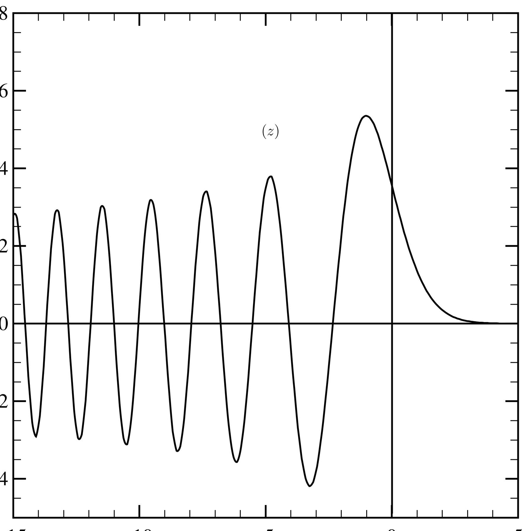
The function \Ai(z). — Figure 8:The function $\Ai(z)$ .

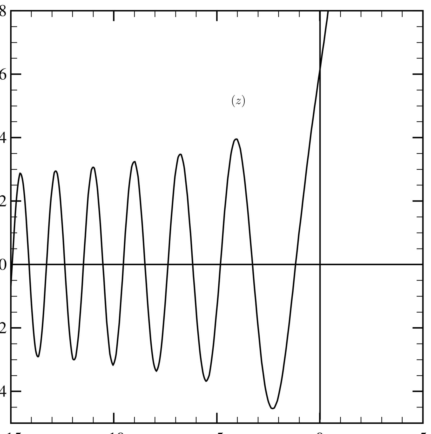
The function \Bi(z). — Figure 9:The function $\Bi(z)$ .

The $\Ai$ and $\Bi$ functions are plotted in Figs.~Figure 8 and Figure 9, respectively. The $\Ai$ function is the solution of Airy’s differential equation (62) that decays exponentially as $z\to\infty$ , and therefore represents the physically allowable solution for a particle in the uniform gravitational field (with zero total energy, since the classical turning point is at $z=0$ ). As seen in Fig.~wkb-8, this function is oscillatory for $z<0$ , with the wavelength and amplitude of the oscillations becoming smaller as $z$ increases in the negative direction, corresponding to the increasing velocity or momentum of the particle falling in the gravitational field. The exponential damping of the function $\Ai(z)$ for $z>0$ corresponds to tunnelling into the classically forbidden region. Finally, the function $\Ai(z)$ shows the characteristic behavior of the wave function at a turning point; the wave function has a large maximum near the turning point, which is a smoothed version of the classical singularity in the probability density. As for the $\Bi$ function, it blows up exponentially in the region $z>0$ , and so is nonphysical for particles in gravitational fields; but we must retain this function for the general WKB problem. For $z<0$ , the function $\Bi(z)$ oscillates like the $\Ai$ function, but $90\deg$ out of phase.

Altogether, the general solution of the Schr"odinger equation (42) in the neighborhood of a turning point has the form,

\psi_tp(x) = c_a \Ai(z) + c_b \Bi(z),

(63)

where $c_a$ and $c_b$ are a new pair of constants, and $x$ and $z$ are related by (60). We must now connect this solution with the solution $\psi_I(x)$ to the left, and $\psi_II(x)$ to the right.

First, working to the left, we invoke the asymptotic forms for the $\Ai$ and $\Bi$ functions for large negative $z$ ,

\begin{aligned} \Ai(z) &= {1\over \sqrt{\pi} \, (-z)^{1/4}} \cos\alpha(z), \qquad z\ll0, \end{aligned}

(64)

\begin{aligned} \Bi(z) &= {1\over \sqrt{\pi} \, (-z)^{1/4}} \sin\alpha(z), \qquad z\ll0, \end{aligned}

(65)

where

\alpha(z) = -{2\over 3} (-z)^{3/2} + {\pi\over 4}.

(66)

Notice that $-z$ is positive in this region. Thus, we can write the wave function at the left of the turning point region in the form,

\psi_tp(x) = {1\over 2\sqrt{\pi} \, (-z)^{1/4}} \bigl[ (c_a - ic_b) e^{i\alpha(z)} +(c_a + ic_b) e^{-i\alpha(z)} \bigr].

(67)

Compare this to the WKB solution in the classically allowed region, (53), which we write in the form,

\psi_I(x) = {1\over \sqrt{p(x)}} \bigl[ c_r e^{i\varphi(x)} + c_\ell e^{-i\varphi(x)} \bigr],

(68)

where

\varphi(x) = {S(x)\over\hbar} + {\pi\over 4}.

(69)

Equations~(67) and (68) must represent the same function. Furthermore, since the waves travelling to the left and right are linearly independent, the left and right travelling waves in the two equations must independently be equal. To show that this is true and to find the connections between the coefficients $(c_r,c_\ell)$ and $(c_a,c_b)$ , we first approximate the momentum function $p(x)$ near the turning point according to (58),

p(x) = \sqrt{2m[E-V(x)]} = \sqrt{-2mV'(x_r)(x-x_r)}= {\hbar\over a} (-z)^{1/2},

(70)

where we use (60) and (61). This shows that the amplitude factors in (67) and (68) are proportional, as they should be. Next, we integrate $p(x)$ to find the action,

{S(x)\over \hbar} = {1\over\hbar} \int_{x_0}^x p(x')\,dx' = \int_0^z (-z')^{1/2} \, dz' = -{2\over3}(-z)^{3/2},

(71)

which shows that $\alpha(z)=\varphi(x)$ . Thus, the phases in (67) and (68) are identical. Now we can read off the necessary relations between the coefficients, which are

\begin{aligned} {1\over 2\sqrt{\pi}}(c_a - ic_b) &= \sqrt{\ds{\ds a \over \ds \hbar}} \, c_r, \end{aligned}

(72)

\begin{aligned} {1\over 2\sqrt{\pi}}(c_a + ic_b) &= \sqrt{\ds{\ds a \over \ds \hbar}} \, c_\ell. \end{aligned}

(73)

This completes the connection between the classically allowed region and the turning point region.

To connect to the right, that is, between the turning point region and the classically forbidden region, we invoke the asymptotic forms of the $\Ai$ and $\Bi$ functions for large positive $z$ ,

\begin{aligned} \Ai(z) &= {1\over 2\sqrt{\pi} \, z^{1/4}} e^{-\beta(z)}, \qquad z\gg0, \end{aligned}

(74)

\begin{aligned} \Bi(z) &= {1\over \sqrt{\pi} \, z^{1/4}} e^{+\beta(z)}, \qquad z\gg0, \end{aligned}

(75)

where

\beta(z) = {2\over 3} z^{3/2}.

(76)

Thus, the wave function to the right of the turning point region has the form,

\psi_tp(x) = {1\over 2\sqrt{\pi} z^{1/4}} \bigl[ c_a e^{-\beta(z)} + 2c_b e^{+\beta(z)} \bigr],

(77)

whereas the WKB solution in the classically forbidden region, (56), has the form,

\psi_II={1\over \sqrt{|p(x)|}} \bigl[ c_g e^{\kappa(x)} + c_d e^{-\kappa(x)} \bigr].

(78)

where

\kappa(x) = {1\over\hbar} K(x).

(79)

As before, (77) and (78) must represent the same function. That the amplitudes are proportional is shown as before, for close to (but to the right of) the turning point we have

|p(x)| = \sqrt{2mV'(x_0)(x-x_0)} = {\hbar\over a} z^{1/2}.

(80)

As for the action integral, we have

\kappa(x) = {1\over\hbar}\int_{x_0}^x |p(x')|\,dx' = \int_0^z z^{\prime\,1/2}\, dz' ={2\over3} z^{3/2} = \beta(z).

(81)

Therefore again we can read off the relations between the coefficients, which are

\begin{aligned} {c_a\over 2\sqrt{\pi}} &= \sqrt{\ds{\ds a \over \ds \hbar}} \,c_d, \end{aligned}

(82)

\begin{aligned} {c_b\over\sqrt{\pi}} &= \sqrt{\ds{\ds a \over \ds \hbar}} \,c_g. \end{aligned}

(83)

Finally, we can eliminate $(c_a,c_b)$ between (73) and (83), and find the desired connection rules between the coefficients $(c_r,c_\ell)$ in the classically allowed region I, and the coefficients $(c_g,c_d)$ in the classically forbidden region II.

The Connection Rules¶

We now summarize the connection rules, first for the case of the classically allowed region to the left of the turning point. This is the case analyzed in Classically Allowed Region to the Left. The potential is sketched in Figure 7, with turning point $x_r$ .

In region I, the classically allowed region where $x<x_r$ and $E>V(x)$ , $p(x)$ is real and positive and is given by (49). The action $S$ is given by (52), which we now write with a slight change of notation,

S(x,x_r) = \int_{x_r}^x p(x') \, dx',

(84)

indicating both limits of the integral. The action $S(x,x_r)$ is real, negative, and increasing to the right in region I. The wave function (53) is now written as

\psi_I(x) = {1\over\sqrt{p(x)}} \Bigl( c_r \, e^{i[S(x,x_r)/\hbar +\pi/4]} + c_\ell \, e^{-i[S(x,x_r)/\hbar +\pi/4]} \Bigr),

(85)

In region II, the classically forbidden region where $x>x_r$ and $E<V(x)$ , $p(x)$ is purely imaginary and is given by (49). Note that

p(x) = i |p(x)|

(86)

in this region. The tunneling action is defined by

K(x,x_r) = \int_{x_r}^x |p(x')|\,dx',

(87)

which differs from (54) in that we now specify explicitly the lower limit of integration. In region II $K(x,x_r)$ is real, positive, and increasing to the right. The wave function in this region is now written as

\psi_II(x) = {1\over \sqrt{|p(x)|}} \Bigl( c_g \, e^{K(x,x_r)/\hbar} + c_d \, e^{-K(x,x_r)/\hbar} \Bigr).

(88)

The connections between the coefficients in regions I and II are given by

\begin{aligned} \begin{pmatrix}c_g\\ c_d\\\end{pmatrix}= \begin{pmatrix}i&-i\\ 1/2&1/2\\\end{pmatrix} \begin{pmatrix}c_r\\ c_\ell\\\end{pmatrix}, \end{aligned}

(89)

\begin{aligned} \begin{pmatrix}c_r\\ c_\ell\\\end{pmatrix}= \begin{pmatrix}-i/2&1\\ i/2&1\\\end{pmatrix} \begin{pmatrix}c_g\\ c_d\\\end{pmatrix}. \end{aligned}

(90)

Next we consider the case of the a turning point separating a classically forbidden region (III) to the left, and a classically allowed region (IV) to the right, as illustrated in Figure 10. The turning point is $x_\ell$ , which is not to be confused with the turning point $x_r$ in Figure 7. The analysis of this case is similar to what we did in Classically Allowed Region to the Left, so we shall skip all details and simply quote the results.

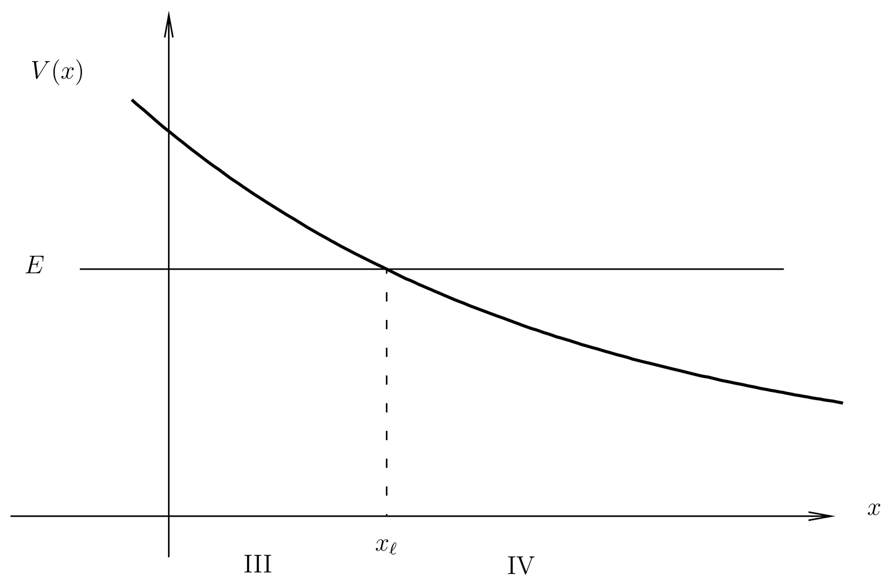
A 1-dimensional potential V(x) falling to the right. Point x_\ell is a classical turning point. — Figure 10:A 1-dimensional potential $V(x)$ falling to the right. Point $x_\ell$ is a classical turning point.

In classically forbidden region~III, we have $x<x_\ell$ and $E<V(x)$ , function $p(x)$ is given by (49) and is pure imaginary, and we define

K(x,x_\ell) = \int_{x_\ell}^x |p(x')| \, dx',

(91)

which is real, negative, and increasing to the right. The WKB wave in this region is

\psi_III(x) = {1\over \sqrt{|p(x)|}} \Bigl( c_g \, e^{K(x,x_\ell)/\hbar} + c_d \, e^{-K(x,x_\ell)/\hbar} \Bigr),

(92)

where $c_g$ and $c_d$ are the coefficients of the waves growing and damping to the right, respectively.

In classically allowed region~IV, we have $x>x_\ell$ and $E>V(x)$ , function $p(x)$ is given by (49) and is real and positive, and we define

S(x,x_\ell) = \int_{x_\ell}^x p(x')\,dx',

(93)

which is real, positive, and increasing to the right. As above, we have explicitly indicated the lower limit of integration $x_\ell$ (different from that in (84). The WKB wave function in this region is

\psi_IV(x) = {1\over \sqrt{p(x)}} \Bigl( c_r \, e^{i[S(x,x_\ell)/\hbar-\pi/4]} + c_\ell \, e^{-i[S(x,x_\ell)/\hbar-\pi/4]} \Bigr),

(94)

where $c_r$ and $c_\ell$ are the coefficients of waves travelling to the right and left, respectively. Notice that the phases $e^{\pm i\pi/4}$ have been introduced with the opposite sign in comparison to (85); this is more convenient for matching the asymptotic forms of the Airy functions in the turning point regions.

The connections between the coefficients in regions III and IV is given by

\begin{aligned} \begin{pmatrix}c_g\\ c_d\\\end{pmatrix}= \begin{pmatrix}1/2&1/2\\ -i&+i\\\end{pmatrix} \begin{pmatrix}c_r\\ c_\ell\\\end{pmatrix}, \end{aligned}

(95)

\begin{aligned} \begin{pmatrix}c_r\\ c_\ell\\\end{pmatrix}= \begin{pmatrix}1&i/2\\ 1&-i/2\\\end{pmatrix} \begin{pmatrix}c_g\\ c_d\\\end{pmatrix}. \end{aligned}

(96)

The principal limitation of these formulas is that they cannot be used when two turning points are too close together, for example, when the energy is too close to the top of a potential barrier. The latter case is important in practice, and can be handled by extensions of the WKB method that are beyond the scope of this course.

A Scattering Problem¶

As a first example of the connection rules, let us consider a one-dimensional scattering problem in which a particle of energy $E$ comes in from the left, encounters an impenetrable potential barrier, and reflects back to the left. As sketched in Figure 11, the potential $V(x)$ approaches zero as $x\to -\infty$ and goes to $\infty$ as $x\to+\infty$ . The particle cannot penetrate the barrier, so all particles launched from the left reflect and go back to the left. The orbit in phase space is illustrated in Figure 12.

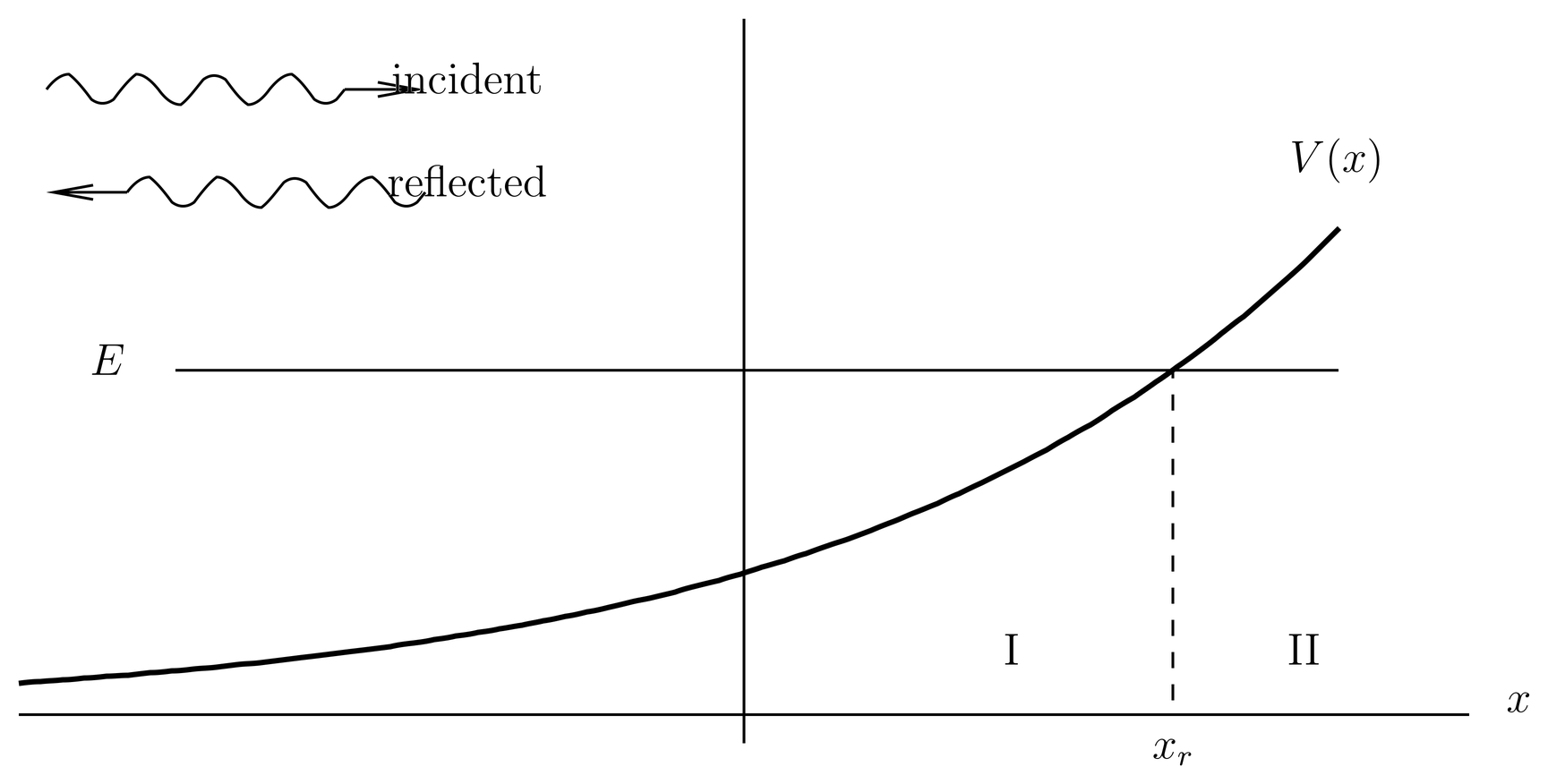
Particle scattering from an impenetrable barrier. Point x_r is the turning point at energy E. Regions I and II are the classically allowed and forbidden regions, respectively. — Figure 11:Particle scattering from an impenetrable barrier. Point $x_r$ is the turning point at energy $E$ . Regions I and II are the classically allowed and forbidden regions, respectively.

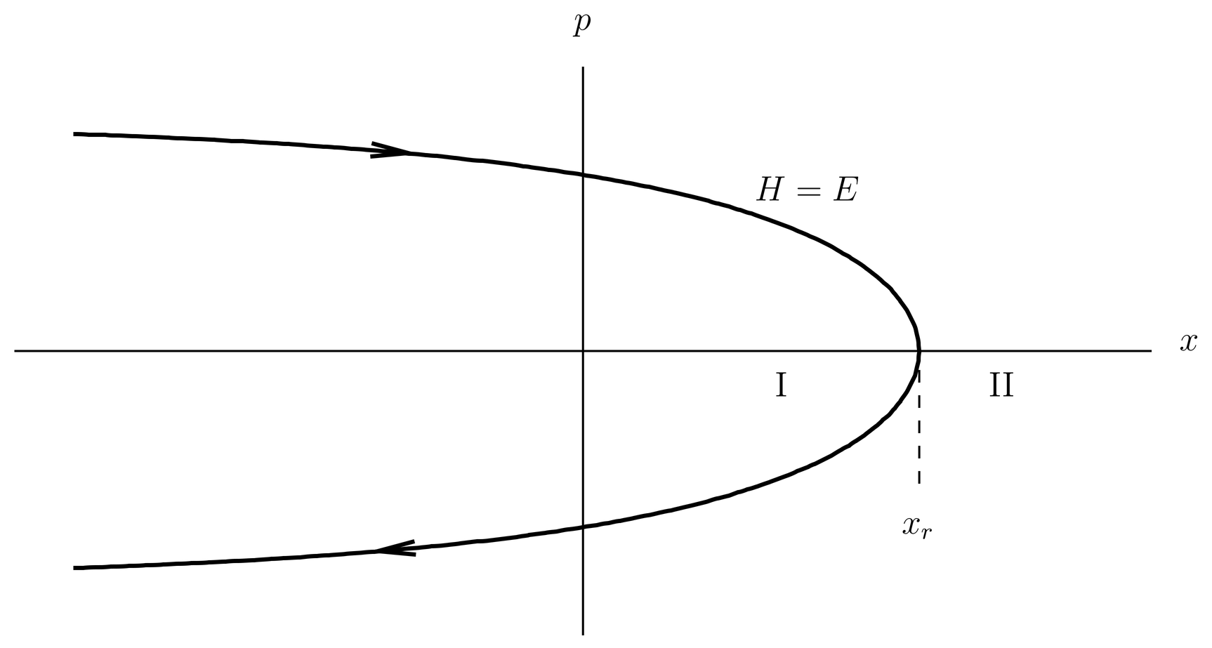
Phase space plot for potential in . Arrows show direction of motion on orbit H=E. — Figure 12:Phase space plot for potential in Figure 11. Arrows show direction of motion on orbit $H=E$ .

To solve the Schr"odinger equation by WKB theory, we observe that the boundary conditions require that the wave function go to zero Region~II, so the coefficient of the growing term $c_g$ in this region must be zero. Let us set $c_d=1$ for the coefficient of the damping term in this region, which amounts to a normalization of the wave function overall. Then applying the connection rule (90), we find the coefficients of the right- and left-travelling waves in the classically allowed Region~I,

\begin{aligned} \begin{pmatrix}c_r\\ c_\ell\\\end{pmatrix}= \begin{pmatrix}-{i\over 2}&1\\ +{i\over 2}&1\\\end{pmatrix} \begin{pmatrix}0\\ 1\\\end{pmatrix} = \begin{pmatrix}1\\ 1\\\end{pmatrix}. \end{aligned}

(97)

Then (85) gives the wave function in Region~I,

\psi_I(x) = {1\over\sqrt{p(x)}} \Bigl(e^{i[S(x,x_r)/\hbar +\pi/4]} + e^{-i[S(x,x_r)/\hbar +\pi/4]} \Bigr) = {2\over\sqrt{p(x)}} \cos\Bigl[{S(x,x_r) \over \hbar} + {\pi\over 4}\Bigr].

(98)

The wave function is an energy eigenfunction of positive energy, in the continuous part of the spectrum. It is nondegenerate, as expected from the fact that $\psi\to 0$ as $x\to+\infty$ . See Degeneracies in One Dimension. It is also real, as expected on the basis of time-reversal invariance. (More precisely, time-reversal invariance requires that the wave function be proportional to a real wave function; in this case, the proportionality factor is real. See The Reality of Energy Eigenfunctions.)

Another way to write the solution is

\psi_I(x) = {e^{i\pi/4}\over\sqrt{p(x)}} \Bigl(e^{iS(x,x_r)/\hbar} + r\, e^{-iS(x,x_r)/\hbar} \Bigr),

(99)

where we define $r$ as the reflection amplitude. For this problem the reflection amplitude is a phase factor,

r=e^{-i\pi/2} = -i.

(100)

A useful way to visualize the reflection amplitude $r$ is to imagine that as the classical particles move along their orbits, they accumulate an action given by

S(t) = \int^t_0 p(t') \, \dod{x(t')}{t'} \, dt'.

(101)

If we let the initial time $t=0$ be the time when the particle reaches the turning point $x=x_r$ , then $S(t)=S(x)$ on the upper branch of the orbit, when $t<0$ , and $S(t)=-S(x)$ on the lower branch of the orbit, where $t>0$ . The function $S(t)$ is a monotonically increasing function for all $t$ , since when $p>0$ , $dx/dt>0$ , and when $p<0$ , $dx/dt<0$ . The upper branch is also the incident wave, while the lower branch is the reflected wave.

Then $S(t)/\hbar$ is the phase of the incident wave in (99) up to the turning point region, whereupon the phase actually loses meaning since the wave there is no longer of WKB form. After the particle emerges from the turning point region, however, the WKB form becomes valid again, but now the phase is $S(t)/\hbar - \pi/2$ . That is, it is as if the particle has suffered a phase shift of $-\pi/2$ on passing through the turning point. This phase shift is also the reflection amplitude, as we have defined it. This is an example of a general rule, that a WKB wave suffers a phase shift of $-\pi/2$ on passing through a turning point.

A turning point is an example of a caustic, which is a generalization of the concept of a focus. When light passes through a focus of a lens, it also suffers a phase shift, but it is $-\pi$ instead of $-\pi/2$ , since the focus involves a two dimensional family of rays.

The one-dimensional version of the probability flux is

J=\Re \Bigl[ \psi^\cc \Bigl(-{i\over m\hbar}\dod{}{x}\Bigr) \psi\Bigr].

(102)

If $\psi$ is a solution of the time-dependent Schr"odinger equation, then the one-dimensional version of the continuity equation is

\frac{\partial \rho}{\partial t} + \frac{\partial J}{\partial x} =0.

(103)

But if $\psi$ is an energy eigenfunction, then $\partial\rho/\partial t=0$ , so $J$ is independent of $x$ .

The incident and reflected waves are the two terms in the WKB solution (99). Each of these is separately a solution of the Schr"odinger equation in the WKB approximation, up to the turning point region where the WKB form breaks down and the waves become strongly coupled with one another. Therefore we can compute the flux for both the incident and reflected waves up to the turning point region, and the values must be independent of $x$ . The easiest place to do the computation is in the asymptotic region $x\to-\infty$ , where the particles are free and the local momentum $p(x)=dS(x)/dx$ is the constant $\sqrt{2mE}$ . We find

J_inc= {1 \over m}, \qquad J_refl = -|r|^2 {1 \over m}.

(104)

Now defining the reflection probability $R$ as the absolute value of the ratio of the reflected flux to the incident flux, we have

R = \left|{J_refl \over J_inc}\right| = |r|^2 =1.

(105)

This is obviously what we expect, since all particles launched from the left must bounce back to the left.

An Oscillator¶

We now apply WKB theory to a one-dimensional bound-state problem. Consider a particle moving in the potential well illustrated in Figure 13. At the energy $E$ , the left turning point is $x_\ell$ and the right one is $x_r$ . We assume the potential rises to infinity to the left of $x_\ell$ and to the right of $x_r$ , so no tunnelling out of the well is possible. Region~I, $x<x_\ell$ , and Region~III, $x>x_r$ , are the classically forbidden regions, while Region~II, $x_\ell < x < x_r$ , is the classically allowed region. Figure 14 shows the orbit $H=E$ in phase space, with arrows indicating the direction of motion.

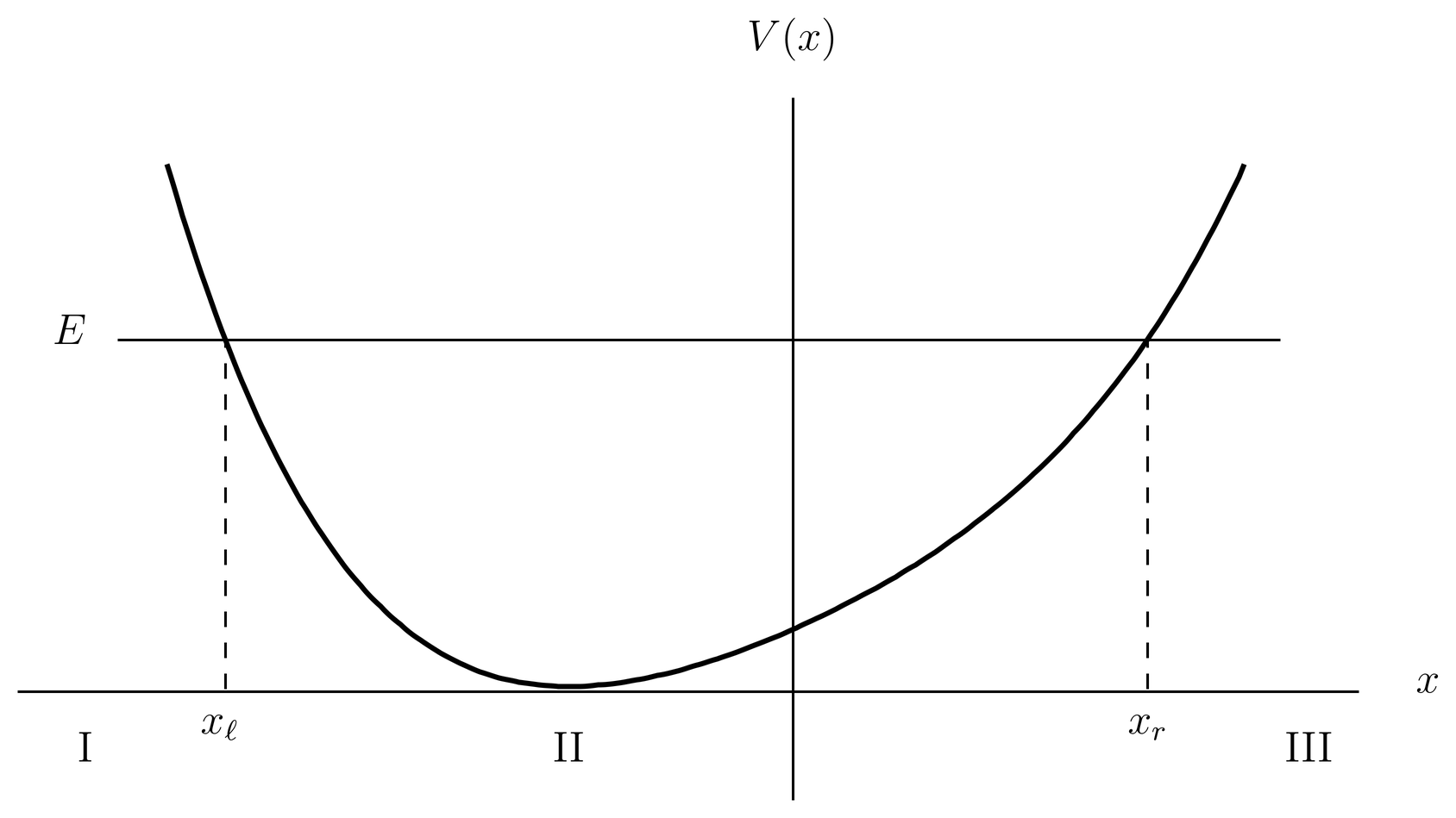
A potential well. There are two turning points at energy E. — Figure 13:A potential well. There are two turning points at energy $E$ .

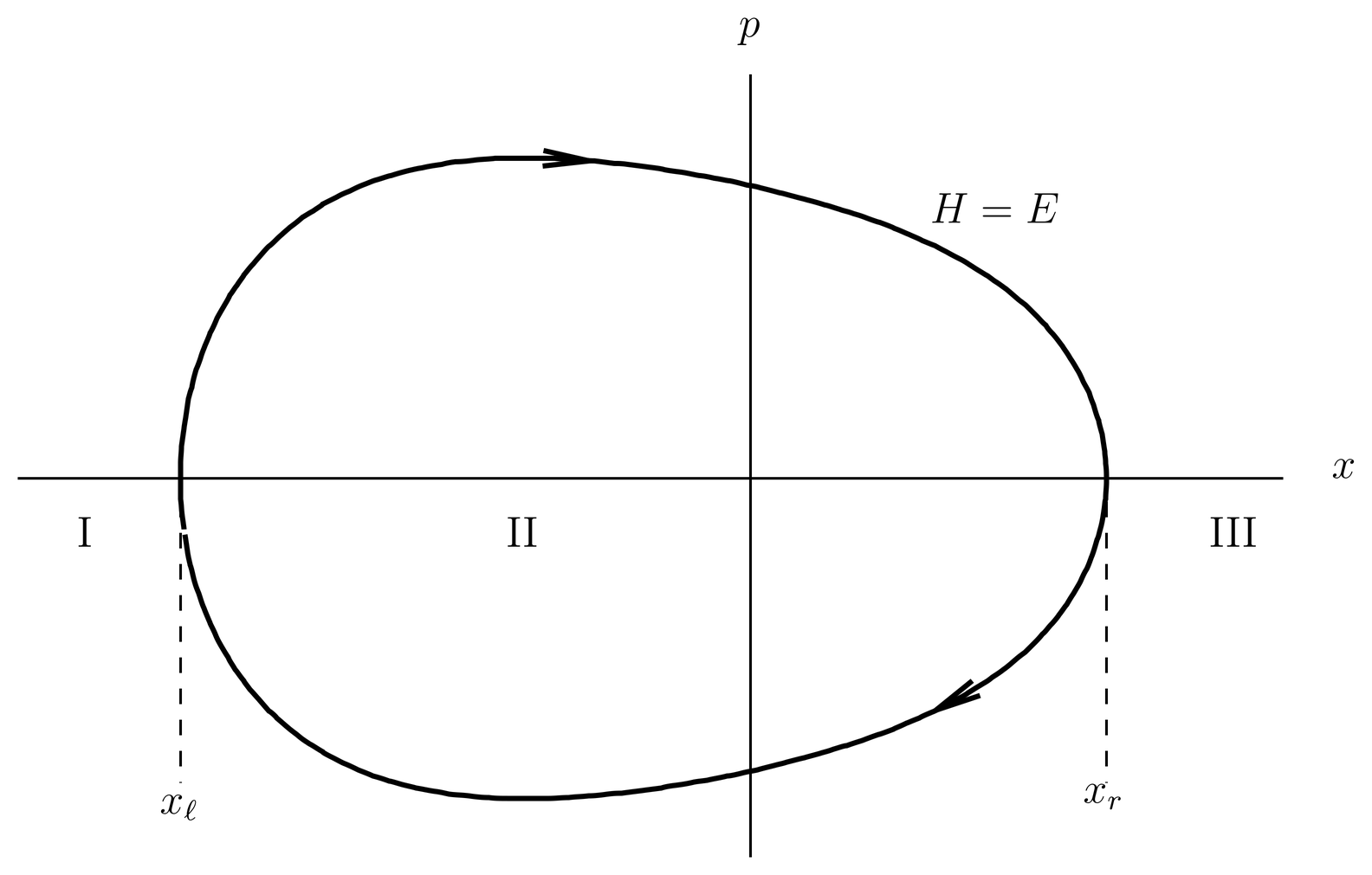
Orbit H=E in phase space for the potential in . — Figure 14:Orbit $H=E$ in phase space for the potential in Figure 13.

Let us begin with a somewhat intuitive approach. The particles accumulate a phase $(1/\hbar)\int p\,dx$ as they move around the orbit, but lose a phase $\pi/2$ when passing through a turning point, so on going completely around the orbit and passing through two turning points the total phase is

{1\over \hbar} \oint p\,dx - \pi.

(106)

Notice that $\oint p\,dx$ is the area in phase space of the orbit. But if the wave function is single-valued, then the phase (106) must be $2n\pi$ , for an integer $n$ . Thus we find

\oint p\,dx = (n+\frac{1}{2})2\pi\hbar.

(107)

Since the area is positive, we have $n=0,1,2,\ldots$ . This is the Bohr-Sommerfeld quantization rule for a one-dimensional oscillator. The discrete set of classical orbits that satisfy this condition are regarded as quantized orbits.

A region of phase space with area $2\pi\hbar$ is sometimes called a Planck cell. The Bohr-Sommerfeld rule says that the $n$ -th quantized orbit encloses $n+\frac{1}{2}$ Planck cells. In particular, the ground state encloses one half of a Planck cell.

In classical mechanics, the quantity

I = {1\over 2\pi} \oint p\,dx

(108)

is called the action of the orbit. (Do not confuse this with other quantities called the “action.”) It depends on the orbit, that is, $I$ is a function of the energy of the orbit, $I=I(E)$ . This function can be inverted to give the energy as a function of the action, $E=E(I)$ . It can be shown (see Prob.~\prbrwkb-1(a)) that

\omega = \dod{E}{I}.

(109)

The Bohr-Sommerfeld quantization rule can be stated by saying that the action is quantized,

I_n = (n+\frac{1}{2})\hbar.

(110)

The quantized values of the action are universal (they apply to all oscillators). The corresponding quantized energies are obtained through the classical action-energy relationship,

E_n = E(I_n).

(111)

These are the energy eigenvalues of a one-dimensional oscillator in the WKB approximation. They are not exact, in general, but they are often good approximations to the true eigenvalues.

To analyze this problem more carefully, and to get the wave functions, we begin by writing down the wave functions in the three regions in terms of a set of unknown coefficients. We have

\begin{aligned} \psi_I(x) &= {1\over \sqrt{|p(x)|}} [a_g \, e^{K(x,x_\ell)/\hbar} + a_d \, e^{-K(x,x_\ell)/\hbar}], \end{aligned}

(112)

\begin{aligned} \psi_II(x) &= {1\over \sqrt{p(x)}} [b_r \,e^{iS(x,x_\ell)/\hbar-i\pi/4} + b_\ell \,e^{-iS(x,x_\ell)/\hbar+i\pi/4}] \end{aligned}

(113)

\begin{aligned} &= {1\over \sqrt{p(x)}} [b'_r \,e^{iS(x,x_r)/\hbar +i\pi/4} + b'_\ell \,e^{-iS(x,x_r)/\hbar -i\pi/4}], \end{aligned}

(114)

\begin{aligned} \psi_III(x) &= {1\over \sqrt{|p(x)|}} [c_g \,e^{K(x,x_r)/\hbar} + c_d \,e^{-K(x,x_r)/\hbar}], \end{aligned}

(115)

where $(a_g,a_d)$ and $(c_g,c_d)$ are the coefficients of the growing and damping waves in Regions~I and III, respectively, and where $(b_\ell,b_r)$ and $(b'_\ell,b'_r)$ are the coefficients of the waves moving to the left and right in Region~II. The wave in region~II is written in two different ways, by referring the action either to the left or the right turning point. (112) is patterned on (92), the unprimed and primed versions of (114) are patterned on (94) and (85), respectively, and (115) is patterned on (88).

To find all the coefficients, we work from the left. In Region~I, boundary conditions require $a_d=0$ , since $e^{-K/\hbar}$ blows up as $x\to -\infty$ . Take $a_g=1$ as a provisional normalization. Then by (96) we have

\begin{aligned} \begin{pmatrix}b_r\\ b_\ell\\\end{pmatrix}= \begin{pmatrix}1&+i/2\\ 1&-i/2\\\end{pmatrix} \begin{pmatrix}1\\ 0\\\end{pmatrix}= \begin{pmatrix}1\\ 1\\\end{pmatrix}. \end{aligned}

(116)

Next we note that the two expressions for the wave in Region~II must be equal, and that

S(x,x_\ell) = \int_{x_\ell}^x p\,dx = \int_{x_\ell}^{x_r} p\,dx + \int_{x_r}^x p\,dx = \pi I + S(x,x_r),

(117)

where we use the fact that

Area = 2\pi I = \oint p\,dx = 2\int_{x_\ell}^{x_r} p(x) \, dx.

(118)

Thus, in Region~II we have

\begin{aligned} &b_r\,e^{i[\pi I+S(x,x_r)]/\hbar -i\pi/4} + b_\ell\, e^{i[-\pi I-S(x,x_r)]/\hbar +i\pi/4} \end{aligned}

(119)

\begin{aligned} &\qquad =b'_r \, e^{iS(x,x_r)/\hbar + i\pi/4} + b'_\ell \, e^{-iS(x,x_r)/\hbar -i\pi/4}. \end{aligned}

(120)

But the right- and left-travelling waves are linearly independent, so this equation can only be satisfied if

\begin{aligned} b_r\, e^{i\pi I/\hbar-i\pi/4} &= b'_r \, e^{i\pi/4}, \\ b_\ell\, e^{-i\pi I/\hbar+i\pi/4} &= b'_\ell \, e^{-i\pi/4}, \\ \end{aligned}

(121)

or, with (116),

\begin{pmatrix}b'_r \\ b'_\ell \\\end{pmatrix} = \begin{pmatrix}e^{i\pi I/\hbar-i\pi/2} \\ e^{-i\pi I/\hbar + i\pi/2}\\\end{pmatrix}.

(122)

Finally, (89) gives

\begin{aligned} \begin{pmatrix}c_g \\ c_d \\\end{pmatrix} = \begin{pmatrix} i & -i \\ 1/2 & 1/2 \\\end{pmatrix} \begin{pmatrix}b'_r \\ b'_\ell\\\end{pmatrix} = \begin{pmatrix}2\cos(\pi I/\hbar)\\ \cos(\pi I/\hbar -\pi/2)\\\end{pmatrix}. \end{aligned}

(123)

But boundary conditions on the right require $c_g=0$ , so

{\pi I \over \hbar} - {\pi \over 2} = n\pi,

(124)

which is equivalent to the Bohr-Sommerfeld rule (107) or (110). Also, we find the coefficient $c_d$ ,

c_d = \cos n\pi = (-1)^n.

(125)

The wave function in the classically allowed region is conveniently written,

\psi_II(x) = {2\over\sqrt{p(x)}} \cos\Bigl[{S(x,x_\ell) \over \hbar} - {\pi\over 4}\Bigr].

(126)

We will leave the normalization of this wave function as an exercise.

Example: The Harmonic Oscillator¶

The harmonic oscillator has the Hamiltonian,

H={p^2\over 2m} + {m\omega^2x^2\over 2},

(127)

so the orbits in phase space are ellipses. The $x$ -intercept of an orbit of energy $E$ is obtained by setting $p=0$ and solving for $x$ ,

x_0 = \sqrt{\ds {\ds 2E \over \ds m\omega^2}},

(128)

and the $p$ -intercept by setting $x=0$ and solving for $p$ ,

p_0 = \sqrt{2mE}.

(129)

The area is

\pi \sqrt{\ds {\ds 2E \over \ds m\omega^2}} \sqrt{2mE} = {2\pi E \over \omega} = (n+\frac{1}{2})2\pi\hbar,

(130)

which we have assigned to the Bohr-Sommerfeld quantized value. Solving for $E$ , we find

E_n = (n+\frac{1}{2})\hbar\omega.

(131)

The WKB approximation to the energy levels of the harmonic oscillator is exact.

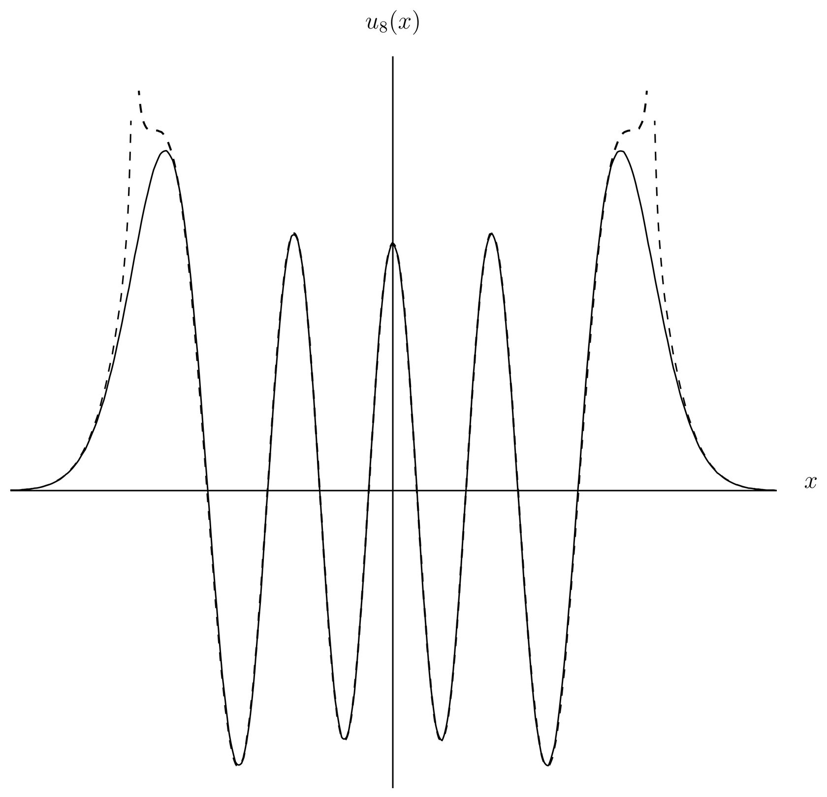
Exact and WKB approximations to the wave function of the harmonic oscillator for n=8. The WKB approximation is the dotted curve, the exact solution is the solid curve. The two are indistinguishable at the scale of the plot except near the turning points, where the WKB solutions diverge. — Figure 15:Exact and WKB approximations to the wave function of the harmonic oscillator for $n=8$ . The WKB approximation is the dotted curve, the exact solution is the solid curve. The two are indistinguishable at the scale of the plot except near the turning points, where the WKB solutions diverge.

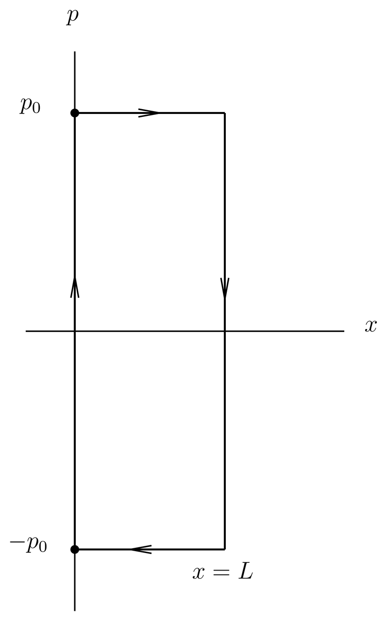
Orbit in phase space for the particle in a box. The particle bounces back and forth between x=0 and x=L with momentum \pm p_0. — Figure 16:Orbit in phase space for the particle in a box. The particle bounces back and forth between $x=0$ and $x=L$ with momentum $\pm p_0$ .

The WKB wave function, however, is only approximate. It is plotted along with the exact wave function for $n=8$ in Figure 15. The WKB wave functions in the figure are those shown in (112), with coefficients determined as in An Oscillator, and with a normalization determined as in Prob.~\prbrwkb-2(a).

Other Types of Turning Points¶

The intuitive idea behind the Bohr-Sommerfeld quantization rule was explained in An Oscillator: as the particle goes around its orbit, it accumulates a phase of $(1/\hbar)\int p\,dx$ , as well as a phase of $-\pi/2$ at each turning point. But if the turning point is at a hard wall, the phase shift is $-\pi$ instead of $-\pi/2$ . That is because $e^{-i\pi}=-1$ , so the reflected wave cancels the incident wave at the wall, where the boundary conditions require $\psi=0$ .

For example, consider the particle in a box, with potential

\begin{aligned} V(x)=\begin{cases}0, & 0\le x \le L, \\ \infty, & x<0 or x>L.\\\end{cases} \end{aligned}

(132)

Let the magnitude of the momentum of the classical particle be $p_0$ , so the particle bounces back and forth with momentum $p=\pm p_0$ . The energy is $E=p_0^2/2m$ . The orbit in phase space is a rectangle with area $2p_0L$ , as shown in Figure 16, so the quantization condition is

{1\over\hbar} \oint p\,dx -2\pi = 2n\pi,

(133)

2p_0L = 2\pi\hbar(n+1).

(134)

Here $n=0,1,\ldots$ so that the orbit will have positive area (the case $n=-1$ gives an orbit of zero energy, which does not correspond to a wave function). We write $N=n+1=1,2,\ldots$ . Then the energy is

E_N = {N^2\hbar^2\pi^2\over 2mL^2},

(135)

the exact answer.

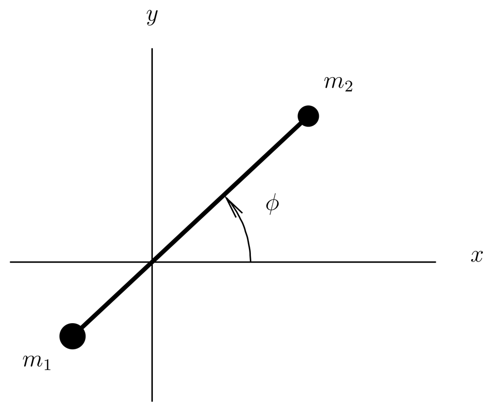
A rigid rotor, consisting of two masses m_1 and m_2 connected by a massless rod, is rotating in the x-y plane. The center of mass is at the origin. — Figure 17:A rigid rotor, consisting of two masses $m_1$ and $m_2$ connected by a massless rod, is rotating in the $x$ - $y$ plane. The center of mass is at the origin.

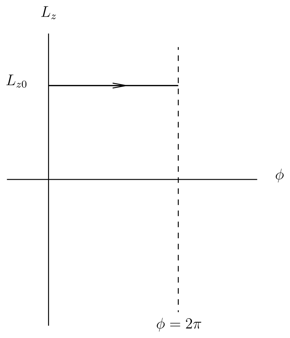
Phase space for a rigid rotor. The orbit has angular momentum L_{z0}. The angle \phi is periodic with period 2\pi. When the orbit reaches \phi=2\pi, it jumps back to \phi=0. — Figure 18:Phase space for a rigid rotor. The orbit has angular momentum $L_{z0}$ . The angle $\phi$ is periodic with period $2\pi$ . When the orbit reaches $\phi=2\pi$ , it jumps back to $\phi=0$ .

For another example, consider a rigid rotor rotating in the $x$ - $y$ plane. See Figure 17. Two masses $m_1$ and $m_2$ are connected by a massless rod. The center of mass is at the origin of the coordinates, and the angle of rotation is $\phi$ . This can serve as a model of the rotations of a diatomic molecule (but real molecules rotate in three-dimensional space, not in a plane).

Let $R$ be the distance between the two masses, and $\mu$ the reduced mass,

{1\over\mu} = {1\over m_1} + {1\over m_2}.

(136)

The moment of inertia is given by

I = \mu R^2.

(137)

To obtain the Hamiltonian we start with the classical Lagrangian, which is just the kinetic energy,

L= {1\over2} I{\dot\phi}^2,

(138)

from which we find the momentum conjugate to $\phi$ ,

p_\phi = \frac{\partial L}{\partial {\dot\phi}} = I{\dot\phi}

(139)

(see (32). This is otherwise the $z$ -component of the angular momentum, so we shall henceforth write $L_z$ instead of $p_\phi$ . The classical Hamiltonian is

H = {L_z^2 \over 2I},

(140)

according to (75).

To quantize this Hamiltonian we notice that the configuration space is a circle with coordinate $\phi$ , so we guess the wave function will be $\psi(\phi)$ , a single-valued function on the circle, that is, a periodic function of $\phi$ . We also guess that $L_z$ , the momentum conjugate to $\phi$ , should be interpreted as the operator $-i\hbar d/d\phi$ . This is a guess based on the Dirac correspondence $p \to -i\hbar d/dx$ in the case of the Cartesian coordinate $x$ . Then the Schr"odinger equation $H\psi = E\psi$ becomes

-{\hbar^2\over 2I} {d^2\psi\over d\phi^2} = E\psi(\phi).

(141)

The normalized eigenfunctions are

\psi_m(\phi) = {e^{im\phi} \over \sqrt{2\pi}},

(142)

where $m=0,\pm1,\pm2,\ldots$ , with energies

E_m = {\hbar^2 m^2\over 2I}.

(143)

These are also eigenfunctions of $L_z$ , with

L_z = m\hbar.

(144)

Now let us solve the same problem by WKB theory. The phase space is the $\phi$ - $p_\phi$ plane, that is, the $\phi$ - $L_z$ plane. See Figure 18. The classical orbit has constant velocity in $\phi$ , that is, constant $L_z$ . The orbit with $L_z = L_{z0}$ is shown in the figure. Since $\phi$ is periodic, when $\phi$ reaches $2\pi$ it jumps back to $\phi=0$ . Now there are no turning points, and the integral $\oint p_\phi\,d\phi$ has the geometrical interpretation of the area between the orbit and the $\phi$ -axis. The quantization condition is

{1\over \hbar} \oint p_\phi\,d\phi = {2\pi L_{z0} \over \hbar} = 2m\pi,

(145)

where $m$ is an integer, without any turning point correction. This amounts to a quantization of $L_z$ ,

L_z = m\hbar,

(146)

where we drop the 0 subscript, which gives the energies (143). The WKB wave functions are also exact.

Planck Cells and Classical Statistical Mechanics¶

In a one-dimensional problem a Planck cell is defined as a region of phase space of area $h=2\pi\hbar$ ( $h$ being Planck’s original constant). The Bohr-Sommerfeld quantization condition (107) amounts to saying that the $n$ -th quantized orbit (counting $n=0,1,\ldots$ ) contains $n+\frac{1}{2}$ Planck cells of area. For large $n$ , this is approximately one Planck cell per quantum state.

In a system with $f$ degrees of freedom the phase space has dimension $2f$ and a Planck cell is defined as a region with a volume $(2\pi\hbar)^f$ . A simple rule is that when the quantum numbers are large, each state occupies a single Planck cell. This rule is asymptotic, which is why we ignore the $1/2$ or other turning point corrections that appear in the one-dimensional Bohr-Sommerfeld condition, or their generalizations to higher dimensional problems.

This rule means that if we have a Hamiltonian $H(x,p)$ , where $x=(x_1,\ldots,x_f)$ and $p=(p_1,\ldots,p_f)$ are $f$ -dimensional vectors, then the number of energy eigenstates with energy less than some energy $E$ is approximately given by the number of Planck cells inside the region $H(x,p) \le E$ in the classical phase space. We denote this number by $N(E)$ , and the stated approximation is

N(E)\approx {1\over(2\pi\hbar)^f} \int_{H(x,p)\le E} d^fx \, d^fp.

(147)

The exact function $N(E)$ is a step function that rises by 1 each time the energy $E$ rises above a nongenenerate energy eigenvalue $E_n$ (or by the degeneracy in the case of a degenerate eigenvalue), while (147) is a smooth approximation to $N(E)$ .

Consider, for example, a free particle confined by hard walls to a region $R$ of three-dimensional configuration space. In this case $f=3$ . The region $R$ need not have any simple shape, such as a box or a sphere. The energy is $\pvec^2/2m$ when $\xvec \in R$ , so the region of phase space where $H\le E_0$ consists of all points $(\xvec,\pvec)$ such that $\xvec \in R$ and

|\pvec| \le p_0=\sqrt{2mE_0}.

(148)

The phase space volume of this region is

\int_R d^3\xvec \int_{|\pvec|\le p_0} d^3\pvec = V {4\pi\over 3} p_0^3,

(149)

where $V$ is the (3-dimensional) volume of $R$ in configuration space and the momentum integral gives the volume of a sphere of radius $p_0$ in momentum space. Thus, according to the rule, the number of energy eigenstates with energy $\le E_0$ is given approximately by

N(E_0) = {4\pi\over 3} {V\over (2\pi\hbar)^3} (2mE_0)^{3/2}.

(150)

This is not counting the spin degrees of freedom of the particle; if the particle has spin $s$ , this number must be multiplied by $2s+1$ .

By differentiating (150) with respect to energy we obtain the density of states,

\dod{N}{E} = {V\over(2\pi\hbar)^3} 4\pi m \sqrt{2mE}.

(151)

This formula is useful in statistical mechanics where it is usually derived for a particle in a three-dimensional box. It actually applies (in an asymptotic sense) to a region of volume $V$ of any shape.

When physicists refer to the “density of states” they almost always mean the number of states per unit energy interval, as here. But if we ask for the number of states per unit volume in phase space, the answer is $1/(2\pi\hbar)^f$ , where $f$ is the number of degrees of freedom. This is a universal result (independent of the Hamiltonian).

The number of states (147) can be expressed in a slightly different form with the aid of the Heaviside step function. This function is defined by

\begin{aligned} \Theta(x)=\begin{cases}0, & x<0\\ 1. & x\ge0\\\end{cases}, \end{aligned}

(152)

and it satisfies

\dod{}{x}\Theta(x) = \delta(x).

(153)

The number of states function (147) can be written in an alternative form,

N(E) = {1\over(2\pi\hbar)^f} \int d^fx \, d^fp\, \Theta\bigl(E-H(x,p)\bigr),

(154)

where now the integral is taken over all of the $2f$ -dimensional phase space. The $\Theta$ -function is 1 inside the region $H(x,p)\le E$ and 0 outside.

This in turn imples a formula for the density of states,

\dod{N}{E} = {1\over (2\pi\hbar)^f} \int d^fx \, d^fp \, \delta\bigl(E-H(x,p)\bigr),

(155)

which expresses it in terms of the classical Hamiltonian.

These results are useful in statistical mechanics. Consider the partition function,

Z(\beta) = \tr e^{-\beta \Hhat} = \sum_n e^{-\beta E_n},

(156)

where $n$ represents a quantum number or set of quantum numbers, however complex, needed to specify a unique energy eigenstate. (If there are degeneracies, then they are represented in (156) by the repetition of the energy eigenvalue $E_n$ for different values of $n$ .) When the number of degrees of freedom $f$ is greater than 1 or 2, and when the energy is substantially above the ground state, the density of states of most systems becomes quite large and $N(E)$ becomes a very large number. This makes it a good approximation to replace the sum (156) by an integral,

Z(\beta) = \int_{-\infty}^\infty dE \, \dod{N}{E} \, e^{-\beta E},

(157)

where $dN/dE$ is understood to vanish below the ground state energy, so the lower limit of integration can be any energy in that range.

Now we substitute the semiclassical approximation (155), whereupon the energy integral can be done. This gives

Z(\beta) = \int_{-\infty}^\infty dE \, {1\over (2\pi\hbar)^f} \int d^fx \, d^fp \, \delta\bigl(E-H(x,p)\bigr) \, e^{-\beta E},

(158)

Z(\beta)={1\over(2\pi\hbar)^f} \int d^fx \, d^fp \, e^{-\beta H(x,p)}.

(159)

This is the classical approximation to the partition function, which was known, apart from the normalization $(2\pi\hbar)^f$ , before the advent of quantum mechanics.

Problems¶

Problem 1.

In this problem we work with one-dimensional, kinetic-plus-potential Hamiltonians,

H={p^2 \over 2m} + V(x).

(160)

(a) Prove (109) when the motion is governed by the Hamiltonian (160).

(b) A classical charged particle in periodic motion radiates at the frequency $\omega$ of the motion as well as all higher harmonics $k\omega$ , $k=2,3,\ldots$ . In many cases the power radiated at higher harmonics is small, but the general principle holds. This follows from standard methods of classical electromagnetic theory, applied to a particle in periodic motion.

In quantum mechanics, the frequency of the radiation emitted by a particle is $\Delta E/\hbar$ , where $\Delta E$ is the energy difference between an initial and final state. This follows from the Einstein relation $E=\hbar\omega$ for the energy of a photon and the Bohr notion that mechanical systems (atoms etc) have discrete energy levels. This part of the argument was understood in the days of the old quantum theory, well before modern quantum mechanics had been developed.

Consider a one-dimensional oscillator in quantum state $n$ with energy $E_n$ where $n$ is large, and suppose it makes a transition to lower energy level $n-\Delta n$ , where $\Delta n$ is small. Using the Bohr-Sommerfeld quantization rule, show that the frequency of the emitted radiation is approximately a harmonic of the classical frequency $\omega$ at classical energy $E_n$ .

Notice that if the power radiated in higher harmonics of the classical problem is small, it means that the most probable quantum transition is one with $\Delta n=1$ .

Problem 2.

Consider the Bohr-Sommerfeld quantization of a 1-dimensional oscillator in a potential $V(x)$ .

(a) Integrate the square of the WKB wave function $\psi$ between the two turning points to obtain the normalization constant. The wave function blows up at the turning points, but you can do the integral anyway. Write out the normalized wave function. (The damped waves in the classically forbidden regions can be ignored.) Replace $\cos^2$ by the average value $1/2$ in the integrand before doing the integral. Express the normalization constant both in terms of the classical period $T$ and the quantity $\partial E_n/\partial n$ , where $n$ is treated as a continuous quantity.

(b) Now assume the potential well is symmetric, $V(-x)=V(x)$ , with $V(0)=0$ . Show that

|\psi(0)|^2 = {1\over\pi\hbar} \sqrt{{\displaystyle 2m \over \displaystyle E}} \frac{\partial E_n}{\partial n} \cos^2 \left( {n\pi\over2}\right),

(161)

and

|\psi'(0)|^2 = { \sqrt{8m^3E} \over \pi \hbar^3} \frac{\partial E_n}{\partial n} \sin^2 \left( {n\pi\over2} \right).

(162)

Carry your calculations only out to leading order in $\hbar$ .

Problem 3.

Consider the potential energy illustrated in Fig.~\figr\cn.19.

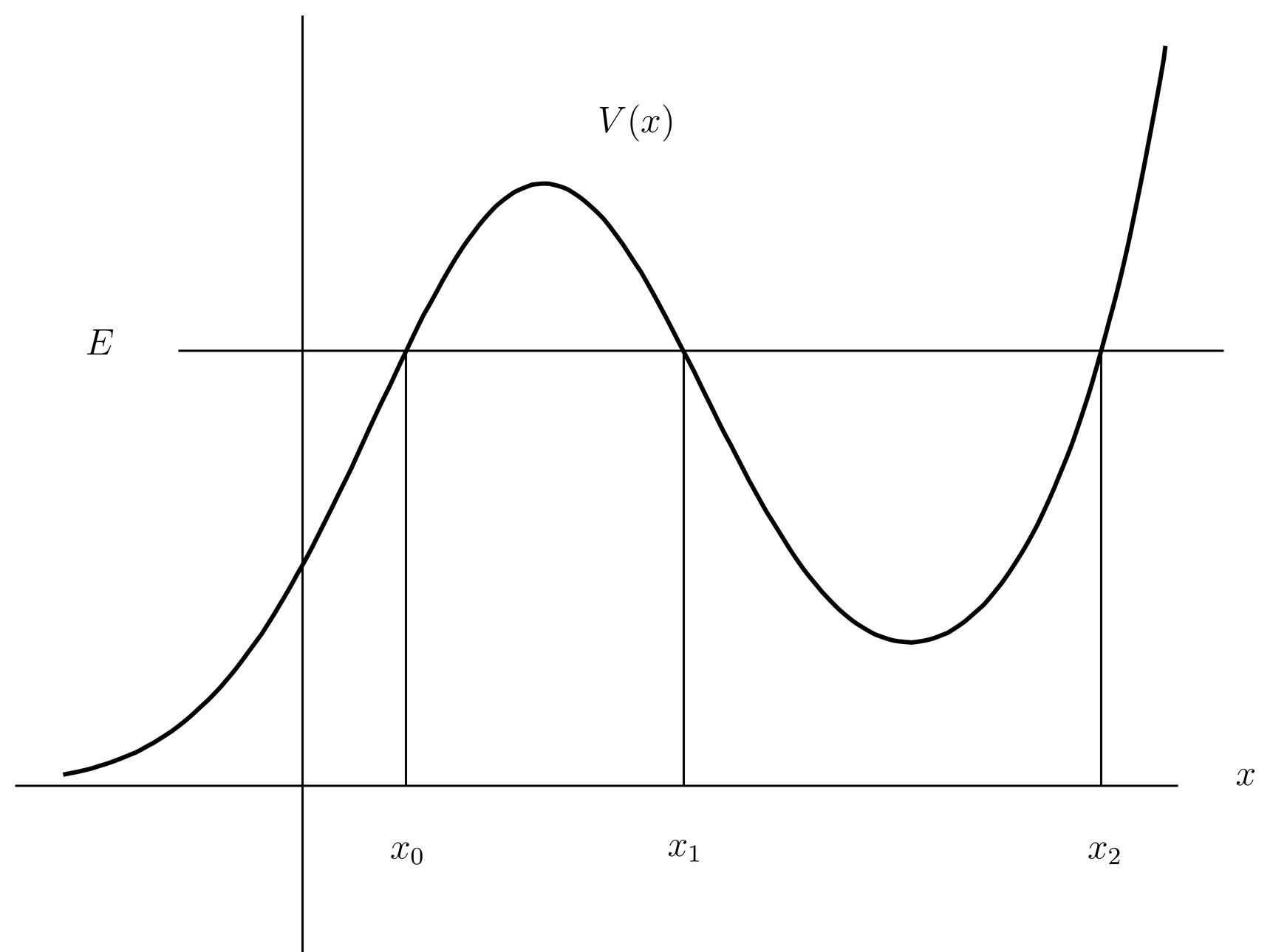
Figure 19:Potential for problem \prbrwkb-3.

For the energy shown, there are three turning points. In the region to the left of $x_0$ let $\psi$ have the form,

\psi(x)={1\over p(x)^{1/2}}\left(e^{iS(x,x_0)/\hbar} +re^{-iS(x,x_0)/\hbar}\right),

(163)

where $r$ is the reflection amplitude. Find $r$ as a function of the energy $E$ . Please use the following notation:

\Phi={2\over\hbar}S(x_2,x_1),

(164)

and

\kappa = {1\over\hbar}K(x_1,x_0).

(165)

Hint: work from right to left.

Show that $|r|^2 =1$ , which means that all particles sent in from the left come back (ingoing and outgoing fluxes are equal). Show that when the energy is not close to a nominal Bohr-Sommerfeld energy level of the well, then $r\approx -i$ (the value $r$ would have if there were no well to the right of $x_0$ ), but that when $E$ increases through such an energy level, then the phase of $r$ rapidly increases by $2\pi$ . This is a resonance. Estimate the range $\Delta E$ over which this change takes place. Assume that the energy is not too close to the top of the well, i.e., the quantity $e^{-\kappa}$ is small.

Estimate the ratio $\psi_in/\psi_out$ of the wave function inside and outside the well, in the case where $E$ is far from a Bohr-Sommerfeld energy level of the well, and in the case where $E$ is equal to one of these energy levels.

Problem 4.

The radial wave equation in 3-dimensional problems with central force potentials looks like a 1-dimensional Schr"odinger equation,

-{\hbar^2\over 2m} {d^2 f\over dr^2} + U(r) f(r) =Ef(r),

(166)

except that $r$ ranges from 0 to $\infty$ , and the potential $U(r)$ is the sum of the centrifugal potential and the true potential $V(r)$ ,

U(r) = {\ell(\ell+1)\hbar^2 \over 2mr^2} + V(r).

(167)

See 16. Central Force Motion. Therefore one-dimensional WKB theory can be applied to the radial wave equation. It can be shown that more accurate results are obtained in the WKB treatment if the quantity $\ell(\ell+1)$ in the centrifugal potential is replaced by $(\ell+\frac{1}{2})^2$ . This is called the Langer modification. Just accept this fact for the purposes of this problem; the justification has to do with the singularity of the centrifugal potential as $r\to0$ .

(a) Take the case of a free particle, $V(r)=0$ . Find the WKB solution in the classically allowed region. For boundary conditions in the classically forbidden region near $r=0$ , just assume that there is only a growing wave (as $r$ increases). Evaluate all functions explicitly; use the abbreviation $k=\sqrt{2mE}/\hbar$ . Take the limit $r\to\infty$ , and reconcile the result with the asymptotic forms of the spherical Bessel function $j_\ell(\rho)$ , quoted by Sakurai in his Eq.~(A.5.15). (Sakurai’s $\rho=kr$ .)

(b) Consider a potential $V(r)$ which is not zero, but which approaches 0 as $r\to\infty$ . Since the particle approaches a free particle as $r\to\infty$ , we might expect the solution at large $r$ to look like a free particle solution, but with a phase shift. Explicitly, if the free particle solution has the form $f(r) = \cos(kr +\alpha_f)$ as $r\to\infty$ , where $\alpha_f$ is the phase shift for the free particle, and the solution in the presence of the potential has the form $f(r) = \cos(kr +\alpha_p)$ as $r\to\infty$ , where $\alpha_p$ is the phase shift in the presence of the potential, then we define $\delta=\alpha_p-\alpha_f$ as the phase shift in the potential scattering, measured relative to the phase shift of a free particle. Use WKB theory to write down an expression for $\delta$ , which will involve the limit of a certain quantity as $r\to\infty$ .

(c) Does this limit exist? It can be shown that it does if $V(r)$ falls off more rapidly as $r\to\infty$ than the centrifugal potential, i.e., more rapidly than $1/r^2$ ; the limit also exists when the true potential falls off exactly as fast as the centrifugal potential, i.e., as $1/r^2$ . Therefore consider the case that $V(r)$ approaches 0 as $1/r^\alpha$ , where $0< \alpha < 2$ . Show that the phase shift exists only if $1 < \alpha < 2$ . In particular, in the important case of the Coulomb potential ( $\alpha=1$ ), the phase shift does not exist (the asymptotic form of the radial wave function $f$ is more complicated than a phase-shifted free particle solution).

Problem 5.

Consider a quantum particle bouncing off the floor. The vertical coordinate is $x$ , and $V(x)=mgx$ . The floor at $x=0$ acts like a hard wall.

(a) Write down the Schr"odinger equation and solve it in terms of Airy functions. Let $z_n$ be the $n$ -th root of the Airy function, that is, $\Ai(z_n)=0$ , where the roots satisfy

\ldots < z_2 < z_1 < z_0 < 0.

(168)

Express the energy eigenvalues as a dimensionless multiple of the reference energy,

K = \Bigl({mg^2\hbar^2\over 2}\Bigr)^{1/3}.

(169)

(b) For the classical bouncing ball, sketch the orbits in phase space. Let $h=E/mg$ be the height to which the ball bounces (but don’t confuse $h$ with $\hbar$ ). Find the Bohr-Sommerfeld approximations to the energy eigenvalues $E_n$ , $n=0,1,\ldots$ . Express your answer as a dimensionless multiple of $K$ . The first three zeroes of the Airy function are -2.33811, -4.08795 and -5.52056. Compare the Bohr-Sommerfeld approximation to the exact eigenvalues for the first three eigenstates.

Problem 6.

Consider the isotropic harmonic oscillator in two dimensions,

H={p_x^2 + p_y^2 \over 2m} + {m\omega^2\over 2}(x^2+y^2).

(170)

Let the number of energy levels less than or equal to a given energy $E$ be $N(E)$ . Degenerate energy levels are counted with their multiplicity. This is a function that increases in steps, but a continuous approximation to it can be obtained by the rule that each quantum state occupies a single Planck cell, as explained in Planck Cells and Classical Statistical Mechanics. Evaluate the integral,

\int d^2\xvec \, d^2\pvec

(171)

over the region $H(\xvec,\pvec)\le E$ to find an estimate for $N(E)$ .

Next, given that $E$ is exactly an energy eigenvalue, evaluate $N(E)$ exactly, and compare to the estimate.

Problem 7.

Let $S(\xvec)$ be a solution of the Hamilton-Jacobi equation (\eqr\cn.25), and define a momentum field $\pvec=\pvec(\xvec)=\del S(\xvec)$ , as in Eq.~(\eqr\cn.10). The Hamiltonian for this problem is Eq.~(\eqr\cn.2). In terms of the momentum field we define a velocity field,

\vvec=\vvec(\xvec)={\pvec(\xvec) \over m},

(172)

This velocity field is similar to the velocity field of a fluid, which is associated with stream lines. As described in the notes, we think of space as being filled with a swarm of particles, in which the particle at position $\xvec$ has velocity $\vvec(\xvec)$ and momentum $\pvec(\xvec)$ .

Let $\xvec_0$ be a fixed point of space, and consider a function $\Xvec(t)$ , defined by

\dod{\Xvec}{t} = \vvec\bigl(\Xvec(t)\bigr),

(173)

with initial coniditions $\Xvec(0)=\xvec_0$ . The function $\Xvec(t)$ defines a stream line of the velocity field. It is also the trajectory of the particle that was at position $\xvec_0$ time $t=0$ , if it follows the velocity field.

Now define the function

\Pvec(t) = \pvec\bigl(\Xvec(t)\bigr),

(174)

so that $\Pvec(t)$ is the value of the momentum field at position $\Xvec(t)$ . Show that

\dod{\Pvec}{t} = -\del V\bigl(\Xvec(t)\bigr).

(175)

This means that the combined functions $\Xvec(t)$ , $\Pvec(t)$ are solutions of the classical Hamilton’s equations, with initial conditions $\Xvec(0)=\xvec_0$ and $\Pvec(0)=\pvec(\xvec_0)$ .

The conclusion is this: If the ensemble of classical particles implied by $S(\xvec)$ is allowed to evolve in time according to the classical Hamilton’s equations, then the condition that the particle at position $\xvec$ has momentum $\pvec$ , which holds at $t=0$ , continues to hold for all time. This fact is more dramatic and amazing in multidimensional problems than it is in one dimension, which is why we presented the three-dimensional version of WKB theory first in these notes.

Problem 8.

The Coulomb potential in the hydrogen atom is $V(r)=-e^2/r$ . It has an infinite number of bound states, but other potentials have only a finite number. The bound energy levels in the hydrogen atom are

E_n=-{me^4\over 2\hbar^2 n^2},

(176)

and they are $n^2$ -fold degenerate. See 17. Hydrogen and Hydrogen-Like Atoms. The principal quantum number $n$ takes on the values $n=1,2,\ldots$ .

(a) Using the method of Planck Cells and Classical Statistical Mechanics, estimate the number of energy levels less than a given energy $E$ , where $E<0$ . Do this in the following way. You need to evaluate the integral,

\int_{H(\xvec,\pvec)\le E} d^3\xvec\,d^3\pvec,

(177)

where

H(\xvec,\pvec)={\pvec^2\over 2m} -{e^2\over r}.

(178)

This is an integral over a 6-dimensional region of the classical phase space. First let $R$ be the region of 3-dimensional $\xvec$ -space over which the kinetic energy $\pvec^2/2m$ can be $\ge 0$ , when $H\le E$ . This will be sphere of some radius $r_0$ , which depends on the energy $E$ . Let $\xvec$ be a point inside $R$ , and let $p_0(\xvec)$ be the maximum value of $|\pvec|$ at that point, corresponding to the maximum kinetic energy allowed at that point for the given value of $E$ . Then the integral (177) can be written,

\int_{r\le r_0} d^3\xvec \int_{p\le p_0(\xvec)} d^3\pvec.

(179)

Since we are only interested in $E<0$ I suggest you define $K=-E$ so that $K=|E|>0$ . This will help avoid sign errors.

(b) Now take the exact energy levels (176), and let $\nu$ be an estimate for the energy level that most closely satisfies $E_\nu=E$ . You may assume that $E_1 < E < 0$ , and that $\nu$ is fairly large, since we are only making asymptotic estimates here ( $E_1$ is the ground state energy). Then estimate the sum

\sum_{n=1}^\nu g_n,

(180)

where $g_n$ is the degeneracy of $E_n$ , and compare it to the results of part~(a). You may make the estimate by replacing the sum by an integral.

(c) You will see from this calculation that the reason that the Coulomb potential possesses an infinite number of bound states is that it has a long-range tail, which dies off only as $1/r$ . It does not come from the singularity at $r=0$ . Suppose we have a potential that dies off as $1/r^\alpha$ as $r\to\infty$ , where $\alpha$ is a positive power. This includes the Coulomb potential (for $\alpha=1$ ) as well as potentials that die more or less rapidly than the Coulomb potential. This is only the asymptotic (large $r$ ) form of the potential, we make no assumptions about what the potential does for small $r$ .

For $\alpha>1$ the potential dies off more rapidly than the Coulomb potential, and it’s logical that at some value of $\alpha$ the number of bound states will stop being infinite and will become finite. Find the value of $\alpha$ for which the number of bound states is infinite, but above which the number is finite.

Introduction¶

The WKB Ansatz¶

Equations for SSS and AAA¶

Other Types of Problems¶

Historical and Other Comments on the Hamilton-Jacobi Equation¶

One-Dimensional WKB Problems¶

Classically Allowed Region to the Left¶

The Connection Rules¶

A Scattering Problem¶

An Oscillator¶

Example: The Harmonic Oscillator¶

Other Types of Turning Points¶

Planck Cells and Classical Statistical Mechanics¶

Problems¶

Equations for $S$ and $A$ ¶