31. The Thomas-Fermi Model
Introduction
The Thomas-Fermi model is a relatively crude model of multi-electron atoms that is useful for many purposes in a first approximation. The basic idea is to represent the electron cloud surrounding the nucleus as a zero-temperature, negatively charged, degenerate Fermi-Dirac fluid, which is held in a condition of hydrostatic equilibrium by a balance between pressure gradients and electrostatic forces.
Zero Temperature, Degenerate Electron Gas
The equation of state of a degenerate, zero-temperature electron gas is a standard topic in statistical mechanics, which we now summarize. We begin with a box of volume , into which electrons are placed. We assume that any external potential is sufficiently slowly varying that the electron wave functions in the box can be approximated by plane waves. Then the density of states with respect to electron wave number is
which includes a factor of 2 for the electron spin. We integrate this from to , where is the Fermi wave number, to obtain the number density :
We solve this for to find,
Similarly, we multiply (1) by the kinetic energy for a single electron and integrate from to to get the total kinetic energy of the electrons in the box,
Eliminating between (2) and (4), we express as a function of the “macroscopic” parameters and ,
Finally, using , we obtain the pressure as a function of the number density ,
which is the equation of state at zero temperature.
Fluid Model of Atom
The electron fluid surrounding the nucleus is like the atmosphere of a planet or a star, except that electrostatic forces hold the fluid in rather than gravitational forces. Since the fluid itself carries charge, the force on a fluid element comes from both the nucleus and the other electrons. Since the fluid organizes itself in a rotationally symmetric cloud around the nucleus, the force on a given electron fluid element arises strictly from the nucleus and the electron fluid at smaller radii than the given fluid element. (In actual atoms, the electron cloud is not exactly rotationally symmetric, but it is so in the Thomas-Fermi model.) Obviously, the density and pressure of the electron fluid will increase from small or zero values at large distances from the nucleus to a maximum at the nucleus itself. One of our goals will be to find expressions for the density and pressure as a function of distance from the nucleus.
The net force per unit volume on an element of the electron fluid is the sum of due to the pressure gradient and due to the electric field, where is the electron charge density. These forces must balance each other in equilibrium. Since and , where is the electrostatic potential, we have the condition for hydrostatic equilibrium,
We note that the force per unit volume will be directed outward, since the pressure must increase as we move inward, so the electrostatic force per unit volume must be directed inward. (7) is augmented by the Poisson equation,
where we include the charge density for the nucleus in the final term. In most of the following analysis we will drop this -function term for the nucleus, since it will be understood that we are working at nonzero , where this term vanishes. We will incorporate the effects of the nuclear charge by imposing proper boundary conditions on various quantities as .
Solving the Self-Consistent Equations
Equations~(6), (7) and (8) are three equations in three unknowns , , and . To solve these, we begin by taking the gradient of (6), to obtain
which we combine with (7) to eliminate the pressure. We then find
which we integrate to obtain
where is a constant of integration and where
Before proceeding, we require an interpretation of the constant . Only a partial interpretation can be given at this point, but we can say some things. First, we note that by (3) the left hand side of (11) can be reexpressed,
where is the Fermi momentum. Thus, (13) gives the kinetic energy of an electron at the top of the Fermi sea, and (11) can be written,
The left hand side of this equation is the total energy (kinetic plus potential) for an electron at the top of the Fermi sea, which is the constant . The potential certainly depends on , as does (since it depends on ), but the sum of the two terms on the left is independent of .
Interpretation of Constant 
This constant is the chemical potential of the electron gas, since the chemical potential is defined as the change in the energy of a system when a particle is added, under conditions of constant entropy. In the present case, the entropy is constant because the temperature is zero, and the energy of the additional particle is the energy at the top of the Fermi sea (kinetic plus potential), which is where the additional particle must go because of the Pauli principle. If the chemical potential were not independent of , then electrons would move from one radius to another to equalize it.
Another interpretation of the constant is obtained from a plot of the potential energy . We do not yet have an analytic solution for , but certainly this function goes as for small , where the field of the nucleus dominates, and it must approach zero for large . There are two cases to consider. Letting be the number of electrons in the atom (a change of notation from above, where was the number of electrons in the box), then if we have a positive ion, and if we have a neutral atom. We know that negative ions exist in nature (for example, ), but negative ions cannot be accommodated in the Thomas-Fermi model, for if we ever reach a radius at which the total electron charge is equal to the nuclear charge , then the vector vanishes at that radius, and there can be no hydrostatic equilibrium. Any additional electron fluid beyond that radius will experience both pressure and electrostatic forces directed outward, and will not be bound. Therefore the cases of interest are and . In the case , the potential must fall off at large as , and in the case it must fall off even faster than , since a neutral atom is being left behind. Furthermore, the potential must decrease monotonically as increases, so that the electrostatic force vector be always directed inward. Therefore the potential must look as in Figure 1, at least schematically.
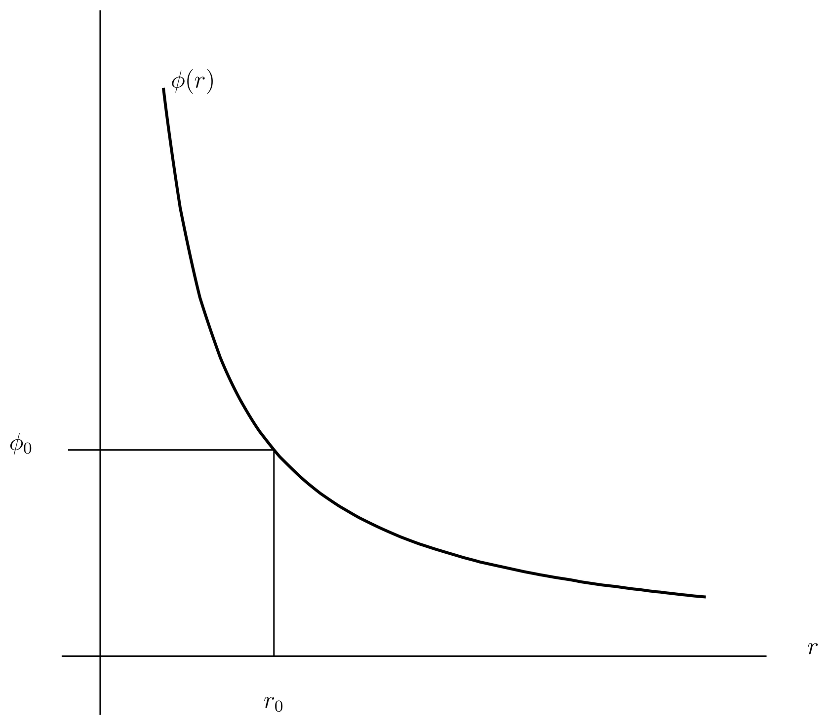
Figure 1:The potential must go to for small and to zero for large , and must decrease monotonically as increases. A positive constant is illustrated, which indicates an atom with a definite radius .
Suppose now that the constant is positive. Then as indicated in the figure, there is some radius where . But at this radius, we have according to (11), which implies according to (6). Therefore the radius must be the surface of the atom, at which the charge density and pressure have fallen to zero, and beyond which there is only vacuum. For , there is no more electron fluid, so the equations above are replaced simply by , , and the Poisson equation for . Later we will see that the case corresponds to a positive ion, . On the other hand, if we let approach zero, then from the figure moves out to infinity, and we have an atom whose electron cloud extends out to infinite radius (the electron density approaches zero, but never exactly equals zero). Later we will see that this case corresponds to a neutral atom, . Finally, we will see later that the case corresponds to a neutral atom under applied pressure.
The Thomas-Fermi Equation
We now rewrite the Laplace equation (8) in terms of the variable ,
which, taken with (11) gives us two equations in the two unknowns and . Neither of these variables is convenient as a dependent variable, because they both diverge at . For example, since is dominated by the field of the nucleus near and since is a constant, we have for small , which by (11) implies that goes as for small .
Therefore instead we introduce a new dependent variable,
which is dimensionless and takes on the value . To express other variables in terms of , we find first
and then
From these it is easy to get a radial equation for . This involves some messy constants, which we clean up by writing
where is a dimensionless radial variable, and where has dimensions of distance and is given by
where is the usual Bohr radius. Finally, this gives the Thomas-Fermi equation for ,
This equation is universal in the sense that all physical constants have been removed by scaling transformations.
Interpreting the Solutions of the Thomas-Fermi Equation
The Thomas-Fermi equation (22) is second order and therefore possesses two constants of integration; but one is taken already by the boundary condition , so there is only a one-parameter family of solutions with physical meaning. This family can be parameterized by , the initial slope of . The Thomas-Fermi equation is nonlinear and cannot be solved analytically, and we must resort to numerical work to find the solutions. Some numerical solutions are plotted in Figure 2 for several values of the initial slope. The character of the solutions can be understood graphically, without doing any numerical work. Note that by (22), as long as and are both positive (the only case of interest), the function must be concave upward.
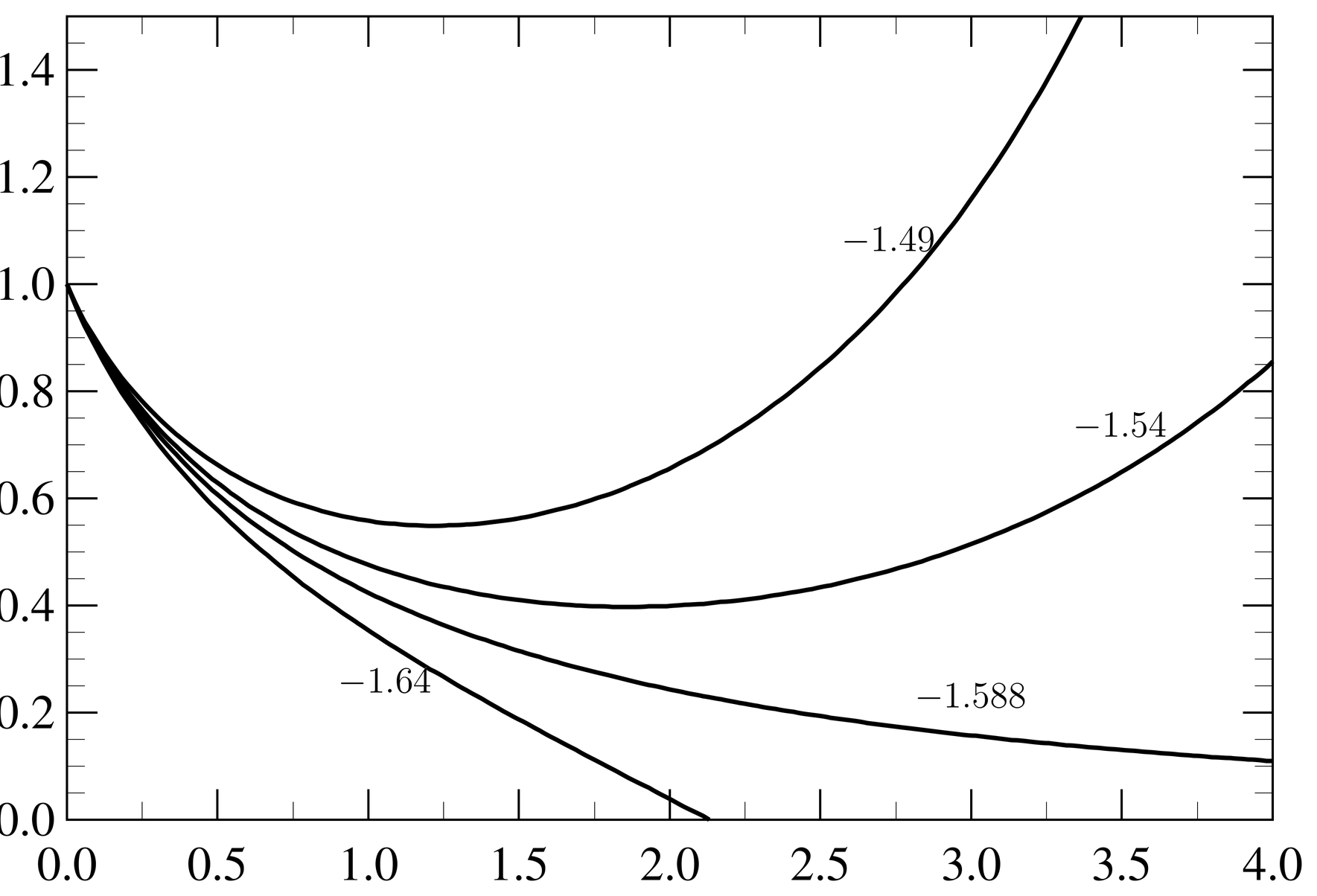
Figure 2:Numerical solutions of the Thomas-Fermi equation for different values of the initial slope. The critical initial slope of about -1.588 corresponds to a neutral atom; initial slopes that are more negative correspond to a positive ion, with a definite radius; and initial slopes that are less negative correspond to a neutral atom under pressure.
There are three cases to consider. In the first case, is sufficiently negative that the curve meets the -axis at some point , so that . The curve in Figure 2 with illustrates this case. Note that the slope is negative. It is clear from the figure that is a function of the initial slope , and that as increases, so does . The meaning of is that it is the surface of the atom, outside of which the electron density vanishes. That is, is the equivalent of the point in Figure 1, according to , for if , then by (17) we also have , and therefore , , and .
In this case it is of interest to compute the total number of electrons in the atom, which is
where we have used (19) and (20). But the integrand of the final integral can be rewritten with the help of the Thomas-Fermi equation (22), whereupon it becomes an exact derivative,
Therefore we have
or,
Since the left hand side is positive, we see that this case corresponds to a positive ion with . If we wish to model a specific positive ion with given values of and , it will be necessary to search numerically for the initial slope that will cause (25) to be satisfied.
As commented earlier, as we increase the initial slope , the value at which increases. It is not obvious but it is true that can be made to increase without bound in this manner, so that as approaches a critical initial slope from below, the curve becomes one that asymptotes to the -axis for large . The critical initial slope is found numerically to be , and the solution in this case is illustrated in Figure 2. As this slope is approached, we have
that is, goes to zero faster than goes to infinity. (In fact, one can show that goes as for large .) By combining (26) and (27), we see that this case corresponds to a neutral atom (), and that such an atom in the Thomas-Fermi model has an infinite radius. For neutral atoms, there is one particular solution of the Thomas-Fermi equation, with and , which applies to all atoms. This solution is a universal function, independent of . This function has been tabulated and can be found in references. We notice that by (20) and (21), we can say that the scale length of the neutral Thomas-Fermi atom goes as .
Finally, the third case is the one in which the initial slope is greater than the critical value of approximately -1.588, so the electron density neither vanishes nor approaches zero at any radius. The curves in Figure 2 with initial slopes and -1.54 illustrate this case. This case can be used to model a neutral atom under pressure; we simply choose the radius at which
and declare that radius to correspond to the volume allotted to an atom in a bulk sample under pressure. Since does not vanish at , there will be a nonzero value of the pressure at , which is interpreted as the applied pressure. In this way it is possible to obtain a crude equation of state for matter under pressure. We do not attempt to model charged ions under pressure, because the large electric fields make it impossible to collect bulk samples of charged ions.
Crudeness of the Thomas-Fermi Model
The Thomas-Fermi model is crude on several accounts. When we derived the equation of state of the degenerate electron gas, we assumed that it was possible to carve out a box that was small enough that the potential was nearly constant over its size, but large enough that it contained a large number of electrons, so that we could take the thermodynamic limit. These requirements are in conflict, and are never satisfied in an atom, except in a crude sense. Furthermore, the electron fluid, as we have treated it, is infinitely divisible, and does not accommodate the discrete charge of individual electrons.
These limitations are obvious in the results, for the Thomas-Fermi model gives no hint of the shell structure that we know exists in atoms. In fact, the Thomas-Fermi model generally does a poor job of describing the properties of the outermost electrons (which are involved in the ionization potential, the chemical properties of the atom, its shell structure, etc.), and of the properties of the electron cloud near the nucleus. (In reality the electron density approaches a finite value as , but in the Thomas-Fermi model it diverges as .) But the Thomas-Fermi model does a fair job of describing the electron density at intermediate radii, and gives moderately good results for the average properties of atoms, such as the average binding energy or rms charge radius. Therefore it is useful for such applications as calculations of the slowing down of particles passing through matter (an important subject in experimental physics). The Thomas-Fermi model is also useful as a starting approximation for more sophisticated atomic models, such as the Hartree-Fock approximation.
Problems
Problem 1.
Let be the solution of the Thomas-Fermi equation (\eqr\cn.22) with initial condition that asymptotes to the -axis as . Assuming that has an expansion in inverse powers of , show that the leading power is , and that
for large }.
Now consider a neutral atom of charge . The Thomas-Fermi solution for a neutral atom predicts a charge cloud which extends to infinity, so if we define the radius of the atom as the radius beyond which there is no more charge, then that radius is always infinite for neutral atoms. But suppose we define the radius of the neutral atom as that radius which contains all the electrons except one. Use the approximation (29) to compute this radius, and note its dependence.
Problem 2.
Consider the Thomas-Fermi model for a neutral atom. There are three contributions to the total energy; they are , the kinetic energy of the electrons; , the potential energy of interaction of the electrons with the nucleus; and , the potential energy of interaction of the electrons with each other.
(a) Show that
where
and where is defined by (21).
(b) The structure equations of the Thomas-Fermi atom can be derived from a variational principle, instead of by balancing forces. To do this, we regard the total energy of the Thomas-Fermi atom as a functional of the electron number density, . The electron fluid is assumed to obey the zero-temperature equation of state of a Fermi-Dirac ideal gas. The particular function that minimizes the total energy, subject to the constraint that the total number of electrons be constant,
is the actual in the Thomas-Fermi model.
Notice that if is replaced by , where is a scale parameter, then the total number of electrons is constant. Use this to show that in the Thomas-Fermi model,