21. Parity
Introduction
We have now completed our study of proper rotations in quantum mechanics, one of the important space-time symmetries. In these notes we shall examine parity, another space-time symmetry. In a latter set of notes we shall take up the third, which is time reversal. All these symmetries are special cases of Lorentz transformations, which are united in a relativistic treatment.
Spatial Inversion
Parity begins life as an operation on three-dimensional, physical space, represented in an inertial frame by the matrix
See also (16) and the discussion in Properties of Rotation Matrices; the Group . This operation, which we call spatial inversion, inverts vectors through the origin, mapping into . The most important properties of for our purposes are
and
for all proper rotations . These properties are trivial in view of (1); in particular, , being a multiple of the identity, commutes with all matrices, so .
The spatial inversion is an example of an improper rotation, that is, it belongs to but not . In fact, every proper rotation is mapped into an improper one by multiplying by , and vice versa. See Fig.~\figr\classrot.5 to visualize the spaces of proper and improper rotations.
Parity in Quantum Mechanics
In this we introduce the operator , called the parity operator, which corresponds to the spatial inversion operation .
Recall that in the case of proper rotations, we sought and found operators , acting on the Hilbert space of various quantum mechanical systems, that implement the effect of classical, proper rotations . The operators were required to satisfy certain postulates, including one that they be unitary, and another that they reproduce the multiplication law of the classical, proper rotations. See Postulates for Rotation Operators. We represent this mapping between classical rotations and rotation operators by
and we say that it specifies a unitary representation of the classical rotation group .
Similarly, in the case of spatial inversion, we seek an operator acting on the Hilbert space of various quantum mechanical systems that is associated with the spatial inversion operation ,
which is required to satisfy certain postulates. These are that be unitary,
and that it should satisfy
and
for all . The latter two postulates are representations of the multiplication laws (2) and (3) at the level of spatial transformations. The first two postulates imply that is both unitary and Hermitian, so that
while the third postulate (8) is equivalent to
where is the angular momentum (the generator of the rotation operators ). In short, is a scalar operator [see (8) and (10)]. These postulates do not uniquely determine the parity operator for all quantum mechanical systems, but they narrow the possibilities considerably so that it is easy to find a suitable definition of in specific cases.
Taken together with the properties of , the postulates for amount to requiring that the set of operators and for form a unitary representation of the full rotation group . That is, generalizing the map (4) to include improper rotations, we can say
Parity for a Spinless Particle in Three Dimensions
Let us begin with the case of a spinless particle moving in three dimensions, for which the basis states can be taken to be the position eigenkets and the Hilbert space is isomorphic to the space of configuration space wave functions . In this case we defined the rotation operators by
which we found satisfactory. See (3) and the discussion in Rotation Operators for Spatial Degrees of Freedom. In a similar spirit, we now guess that the definition of parity for such systems should be
This transformation law on basis kets implies that wave functions transform according to
We must check that this definition satisfies the postulates (6)--(8).
First, by applying twice, we have two changes of sign,
so the postulate (7) is satisfied. Next, since
for all wave functions , the operator is unitary (it preserves the normalization of states), and the postulate (6) is satisfied. See Problem Paragraph(c). Finally, since
we have , which is equivalent to the postulate (8). All postulates are satisfied, so we shall take (13) as the definition of for a spinless particle in three-dimensional space.
As for the last postulate (8) and its equivalent form (10), since the angular momentum for a spinless particle in three-dimensional space is the orbital angular momentum , we have
This follows from the postulates, but can also be verified directly.
It is also of interest to compute the conjugation relations of other vector operators with respect to . We start with the position operator . For the sake of the following demonstration, we will write for the operator, and for associated vectors of -numbers. In the configuration representation, the operator means multiplication of the wave function by the position of the particle, that is,
Now computing the effect of on an arbitrary wave function, we have
where we use .
Thus we have
where we have dropped the hats so that now represents the operator again. We see that conjugating the position operator by converts it into . This is reasonable, in view of the action of on points of space. Similarly, we find
This is fairly obvious, since in the position representation, and should change sign when does. Taking the cross product of (21) and (22), we obtain (18).
Parity for Spin Systems
Next let us consider just the spin degrees of freedom for a particle with spin, ignoring the spatial degrees of freedom for the time being. The Hilbert space is
with the standard angular momentum basis shown. We would like to find a reasonable definition of that satisfies the postulates (6)--(8). This means finding the action of on the basis states . Since the angular momentum in this case is the spin vector , the form (10) of the third postulate is
The states are nondegenerate eigenstates of on the Hilbert space (23), and (24) implies . Therefore by Theorem Theorem, must also be an eigenstate of parity,
where as indicated the eigenvalue might depend on , as far as we know at this point. Theorem Theorem does not tell us the value of this eigenvalue, but it must be real since is Hermitian. Now by applying raising and lowering operators and using (24) again, we have
or, on canceling the square roots,
By comparing this to (25), we see that , or, by induction, that is independent of for all values it can take on. This fact could have been seen from another standpoint, for since is a scalar operator, by the Wigner-Eckart theorem for scalars its eigenvalues must be independent of . See Secs. Energy Eigenstates in Isolated Systems-The Nucleus and the M"ossbauer Effect. Thus we shall write simply
In fact, since the states form a basis for , all kets in this space are eigenstates of with eigenvalue , that is, is times the identity operator.
Now using the fact that , we find that , or , and we have
The postulates required of reduce its definition to a choice of a sign. This sign is the same for all vectors in the Hilbert space of (23), so it is really a characteristic of the particle, that is, a constant like the spin quantum number .
Can this sign be determined by any further arguments or by appeal to experimental results? Within nonrelativistic quantum mechanics, the answer is no, the final choice of sign is without physical consequences and can be made arbitrarily. The simplest choice is , and for as long as we remain with the nonrelativistic theory, we shall assume that the parity operator satisfies
That is, the parity operator has no effect on the spin state of the particle.
In relativistic quantum mechanics, however, it becomes possible to create and destroy particles. In some cases, an initial state of a definite parity decays or otherwise evolves into a state in which a particle has been created or destroyed, and in order to account for conservation of parity it is necessary to attribute a certain parity to a particle because of the kind of particle it is. This is called intrinsic parity, and it is equivalent to making one of the two choice for each type of particle in the process. Some details of this assignment depend on the type of particle, fermion or boson. (It turns out that for fermions, the intrinsic parity of a particle-antiparticle pair is odd; it is arbitrary whether the particle is interpreted as having even intrinsic parity and the antiparticle odd, or vice versa. See 48. Covariance of the Dirac Equation.) Not all interactions conserve parity, but for those that do, it is necessary in relativistic interactions to take into account the intrinsic parities of particles. Then the total parity of a state is the product of the intrinsic parities of the particles times the parities of the spatial parts of the wave functions. For example, the photon turns out to have negative intrinsic parity. This is related to Laporte’s rule, which we discuss presently, which states that the parity of an atom changes when a photon is emitted in an electric dipole transition. The parity of the atom changes, but the parity of the entire system, including the electromagnetic field, is conserved, as we see when we include the intrinsic parity of the photon. The intrinsic parity of particles cannot be understood very well outside of the relativistic theory, but we will have more to say about it 48. Covariance of the Dirac Equation.
Returning to nonrelativistic quantum mechanics, if we include the spatial degrees of freedom of a particle, so that the Hilbert space is spanned by the basis kets
then the parity operator is defined by
This is equivalent to the action on the wave function,
As we say, parity is a purely spatial operator, and does not affect the spin (in the nonrelativistic theory).
Transformation Properties Under Parity
Returning to the conjugation relations (18), (21) and (22), we see that some vectors (for example, and ) change sign when conjugated by parity, while some (for example, and ) do not. All these vectors are vector operators according to the definitions (15) or (21), that is, they all transform in the same way under conjugation by proper rotations, but their transformation laws under improper rotations differ. Thus we can take the set of vector operators and break it down according to how the vectors transform under parity. If is a vector operator and
then we will say that is a true vector or polar vector if the sign is -1, or a pseudovector or axial vector if the sign is +1. Thus, and are true vectors, while and (more generally, any angular momentum ) are pseudovectors. Other vectors in physics can be classified similarly, for example, the electric field is a true vector, while the magnetic field is a pseudovector.
Similarly, we can classify scalars. If is a scalar operator according to the definitions (8) or (10), and if
then we will say that is a true scalar if the sign is +1 or a pseudoscalar if the sign is -1 (notice the signs are reversed compared to the terminology for a vector). An example of a true scalar is , while an example of a pseudoscalar is .
Hamiltonians Invariant Under Parity
We argued previously that the Hamiltonian for an isolated system must be a scalar, that is, invariant under proper rotations, because the energy could not depend on the orientation. See Energy Eigenstates in Isolated Systems. But are these Hamiltonians scalars or pseudoscalars or a combination of the two? That is, are they also invariant under parity?
As an example, consider a central force Hamiltonian,
This certainly commutes with parity, for although is mapped into , the kinetic energy contains , which is invariant. Also, the potential energy is a function of the radius , the magnitude of the vector , which does not change when changes its sign. Parity is a good quantum number for all central force Hamiltonians.
As we know, central force Hamiltonians usually represent a two-particle system interacting by means of forces derivable from a potential that is a function only of the distance between the two particles. See Two-Body Central Force Motion. All these Hamiltonians commute with parity. This generalizes to any number of particles interacting by means of forces derivable from potentials depending only on the distances between the particles, such as the electrostatic Coulomb approximation to the interactions of charged particles. This covers a wide variety of approximate Hamiltonians for atoms, molecules, and other systems. What happens when we include electromagnetic and relativistic effects? As it turns out, such Hamiltonians still commute with parity, as long as the electromagnetic fields are internally generated (that is, the system is still isolated). For example, one of the magnetic and relativistic corrections in a single electron atom is the spin-orbit term, which is proportional to . But by the rules above, this is a true scalar (the dot product of two pseudovectors). What about when we include the emission and absorption of radiation, that is, of photons? In this case, too, parity is conserved, as long as we include the parity of the electromagnetic field (that is, of the photons) in our account. We summarize these facts by saying that the electromagnetic forces conserve parity.
The strong forces, responsible for the interactions of nucleons inside a nucleus as well as interactions of other hadronic particles such as the -meson, also conserve parity. This fact was originally established by experiments involving nuclei and particles, which showed that in strong interactions the parity of the initial state is always equal to the parity of the final state. In reckoning the parity of states, however, it is necessary to take into account the intrinsic parities of various particles, for example, the -meson (all three charge states of it) has negative intrinsic parity (just like the photon).
For these reasons, it used to be believed that parity conservation was a fundamental law of nature, much like the rotational invariance of isolated systems. This belief ended abruptly in 1956, however, when Lee and Yang suggested that parity might be violated in weak interactions. They also suggested experiments to test the idea that were quickly carried out. These showed that, indeed, parity is violated in -decay, a prime example of a weak interaction.
The weak forces are present in ordinary atomic and nuclear interactions, but, as the name implies, they are very small compared to the electromagnetic and strong interactions, at least at low energy. The weak forces become relatively stronger as the energy is increased, and it is currently believed that at energies much higher than now available in accelerators the strong, electromagnetic and weak forces all become comparable in strength. Considering only low energy interactions, however, we can say that the weak interactions are extremely small compared to the electromagnetic and nuclear interactions, in fact, they are so small that they are quite difficult to detect even if one is looking for them. There has been some effort in the Berkeley Physics department to detect the effects of weak interactions in atomic physics, and these experiments are difficult. For most ordinary purposes at ordinary energies, the weak interactions can be ignored and all Hamiltonians for isolated systems conserve parity to an extremely high degree of accuracy.
It is, however, easy to create a system that does not conserve parity, simply by placing it in an external field. Such a system is no longer isolated, and parity need not be conserved. For example, suppose a particle of charge moving in a central force field is placed in an external, uniform electric field . Then the Hamiltonian is
This does not commute with parity because the last term changes sign upon conjugation by parity.
In such cases, however, parity conservation is restored if we enlarge our definition of “the system” to include the charges creating the electric field. For example, if is created by positive and negative charges arrayed along the parallel plates of a capacitor, and if these charges are included in “the system,” then will swap the positive and negative charges and reverse the direction of . Since also changes sign, the whole Hamiltonian will once again be invariant under parity.
Parity and Energy Eigenstates in Isolated Systems
Suppose we have an isolated system with Hamiltonian . As we have explained, in most applications commutes with parity to an extremely high degree of accuracy, so let us assume that , that is, .
Since the system is isolated, commutes with all proper rotations, and is a scalar operator according to the definition (8). Then Theorem Theorem states that the energy eigenspaces consist of one or more irreducible subspaces under rotations, and the addendum says that, with few exceptions, they consist of precisely one irreducible subspace. So let us consider this generic case, for which each energy eigenvalue is associated with a definite value and has an energy eigenspace that is -fold degenerate.
As in 13. Representations of the Angular Momentum Operators and Rotations{} and \transfop{} let be the eigenspace of operators and with quantum numbers and , and let be a bound energy eigenstate in the stretched subspace with eigenvalue , so that
Under our assumptions of genericity, restricted to is nondegenerate, that is, is the only state in with the energy .
Now commutes with and hence with and , and so it can be restricted to . And since is a nondegenerate eigenstate of and since commutes with , according to Theorem Theorem, must also be an eigenstate of parity,
where . Theorem Theorem does not tell us what the value of is.
Now it is easy to show that all the states obtained by applying lowering operators to are also eigenstates of parity with the same eigenvalue as the stretched state. That is,
for . That is, all degenerate energy eigenstates in the irreducible subspace have the same parity.
Thus the parity value can be associated with the energy level itself, just like the value. This is why the three nuclear states shown in Fig.~\figr\transfop.1 are assigned definite values of parity (all three, , and , have negative parity).
In the case of nuclei, the energies, angular momenta (or spins) and parities of energy levels are determined experimentally, since theoretical calculations of these quantities are difficult. In atoms and molecules, theory is in better shape, and these quantities can be calculated with greater or lesser difficulty.
In the nongeneric case of the electrostatic model of hydrogen, it is not true that all energy eigenstates are eigenstates of parity. It is true that in central force motion each angular momentum value is associated with the definite parity [see (52)], but since there are degeneracies of energy that cross angular momentum values, it is possible to form linear combinations of energy eigenstates of the same energy but opposite parity. For example, the and levels in hydrogen have the same energy but opposite parities. These facts play an important role in understanding the Stark effect, which is discussed in 24. The Stark Effect in Hydrogen and Alkali Atoms.
Parity in One-Dimensional Systems
Consider a one-dimensional Hamiltonian,
This commutes with parity if and only if , that is, if the potential is symmetric about . Now in one-dimensional systems with a localized potential, the bound energy eigenstates are nondegenerate because the wave functions must vanish at . See Degeneracies in One Dimension. Therefore by Theorem Theorem, the energy eigenstates must also be eigenstates of parity. That is, the bound energy eigenfunctions satisfy , for some choice of sign that depends on the eigenfunction. For example, in the harmonic oscillator, which has the symmetric potential , the -th energy eigenfunction has parity . See \harmosc.6.
Considerations of Symmetry Raised by Parity
Parity illustrates some issues that arise whenever a Hamiltonian possesses a symmetry. Some of these have already been discussed in connection with rotations, but parity is a simpler symmetry so some of the ideas are easier to appreciate.
Whenever a Hamiltonian possesses a symmetry and we wish to diagonalize it or otherwise study its properties, it is a good idea to diagonalize the symmetry operators first. This is because symmetry operators are usually easier to diagonalize than Hamiltonians, and their eigenbases, sometimes called symmetry-adapted bases, are especially convenient for further study of the Hamiltonian. For example, in the case of rotational invariance, the symmetry adapted basis is the standard angular momentum basis , an eigenbasis of and .
Similarly, if a Hamiltonian commutes with parity, it may be convenient to study it in a basis which is an eigenbasis of parity. Since , the eigenvalues satisfy , or . Thus the Hilbert space is decomposed into two subspaces, the eigenspaces of parity with . We can call these the even and odd subspaces,
Then a symmetry adapted basis consists of an orthonormal basis inside plus an orthonormal basis inside . We can write the basis vectors as , where
so that indicates which subspace the vectors lie in, and where is a label of the orthonormal basis vectors inside (for ) or inside (for ). This notation is similar to the notation which we used for a standard angular momentum basis, where the index plays a similar role.
It is possible to write down projection operators that project onto the even and odd subspaces in terms of the parity operator itself. These are
It is easy to show that the operators satisfy the requirements of a projection operator (see Projection Operators), and that when applied to an arbitrary state (not necessarily an eigenstate of parity), they project it onto one or the other of the two subspaces, producing an eigenstate of parity of the eigenvalue indicated. For example, in a one-dimensional problem, if is an arbitrary wave function (not necessarily even or odd), then
and
are the even and odd parts of , respectively.
The matrix elements of the Hamiltonian in the symmetry adapted basis are noteworthy. Assuming the Hamiltonian commutes with parity, we have
which implies that the matrix element vanishes unless . But this is equivalent to , so the Hamiltonian is diagonal in the parity quantum number , and we have
where just indicates the indices the nonvanishing matrix elements can depend on. This may be compared to (55), which applies to Hamiltonians that are invariant under proper rotations. The fact that the matrix element vanishes if is sometimes stated in words by saying that the Hamiltonian does not “connect” states of different parity.
In many cases it is necessary to diagonalize a Hamiltonian numerically, by setting up a matrix for it in some basis. There is the question, however, of what basis to use. If the Hamiltonian respects a symmetry then there is great advantage in using a symmetry adapted basis, since it reduces the size of the matrices that must be diagonalized. For example, in the parity-adapted basis , to diagonalize a Hamiltonian that commutes with parity we must diagonalize the two matrices with rows and columns indexed by and , for . Effectively we are diagonalizing the Hamiltonian separately in each of the subspaces and . If we arrange the basis vectors so that all the even vectors come first, and all the odd vectors come second, then the Hamiltonian matrix has the form,
where the upper (or even-even) block is the matrix , and the lower (or odd-odd) block is the matrix , and where indicates a non-zero block.
There are many numerical algorithms for diagonalizing a matrix, but a common one (the Householder algorithm) involves a computational effort that scales as , where is the size of the matrix. Thus the effort to diagonalize two matrices of size is , or about the effort of diagonalizing a single matrix. This is the improvement in computational efficiency when using a symmetry adapted basis for a Hamiltonian that commutes with parity, as compared to diagonalizing the Hamiltonian in an arbitrary (nonsymmetric) basis.
Parity and Selection Rules
Parity gives rise to important selection rules which we will illustrate for the case of dipole transitions in an electrostatic model of a single-electron atom. The energy eigenfunctions are the usual ones in central force motion,
which we shall write in ket language as . The matrix elements relevant to electric dipole transitions are
We need to find the action of parity on the eigenstates . Since the radius is invariant under the replacement , only the part of the wave function is affected by parity. The 's have the property that if they are multiplied by , where is the radius, then the result is a homogeneous polynomial in the Cartesian coordinates , and of degree . See 's in Cartesian Coordinates. But since , and all change sign under parity, and since the factor is invariant, the changes by under parity. We summarize this by writing
The energy eigenfunctions (50) are also eigenfunctions of parity, with eigenvalue . This is often a useful fact. Notice that the eigenvalues do not depend on . This was to be expected, since is a scalar operator, and according to the Wigner-Eckart theorem, the eigenvalues of a scalar operator do not depend on . See Energy Eigenstates in Isolated Systems.
Now using the fact that is odd under parity, we can make some statements about the matrix element (51). That is,
Thus, the matrix element (51) vanishes unless , or
where .
We see that the parity of the atomic state must change under an electric dipole transition. This selection rule is known as Laporte’s rule. Initially it was observed experimentally, and later it was explained by Wigner on the basis of parity. As noted above, Laporte’s rule is equivalent to the statement that the intrinsic parity of the photon is negative.
In the case of the matrix element (51), the Wigner-Eckart theorem gives the selection rule , that is, these are the values of allowed by rotational invariance alone. But parity excludes the value , so the final selection rule is .
Problems
Problem 1.
This is essentially Sakurai’s problem 4.4, p.~282 (revised edition), or problem~4.4, p.~300 (second edition), but I’ve rewritten it to make it more clear.
We did not discuss the spin angular functions in class, but these are spinor functions on the unit sphere that arise when we combine orbital and spin angular momentum for a central force problem for a spinning particle. Here we will take the case (for example, in hydrogen). Let be ket language for the wave function , the solution of the Schr"odinger equation for a spinless particle in a central force field, and let be the usual spin states (here and ). We distinguish between and , the two types of magnetic quantum numbers. We multiply the wave functions times the spin functions and form linear combinations with the Clebsch-Gordan coefficients to get eigenstates of and , where . These are
The spatial wave functions factor into a radial part times an angular part. Let us write this in ket language as . The factor or is the same for all terms in the sum above, so it can be taken out and what is left is a two-component spinor that depends only on the angles. This is what in wave function language Sakurai calls ; in ket language we will write
(a) For the case , , , write out the two-component spinor as functions of .
(b) Multiply this by , and express the result as a linear combination of other spin angular functions .
(c) Certain values of , and occur in the sum, and certain others do not. Use symmetry principles to explain why the values that occur are allowed and the others are not.
Hint: It may help to think of three kinds of rotations: spin rotations, orbital rotations, and total (spin plus orbital) rotations.
Problem 2.
This is Sakurai, problem 4.5, p.~282 (revised edition), or problem~4.5, p.~300 (second edition).
Because of weak (neutral-current) interactions, there is a parity-violating potential between the atomic electron and the nucleus as follows:
where and are the spin and momentum operators of the electron, and the nucleus is assumed to be situated at the origin. As a result, the ground state of an alkali atom, usually characterized by , actually contains very tiny contributions from other eigenstates as follows:
On the basis of symmetry considerations alone, what can you say about the values of that give rise to nonvanishing contributions? Suppose the radial wave functions and energy levels are all known. Indicate how you can calculate . Are there any further restrictions on that go beyond those due to symmetry considerations?
Problem 3.
This problem concerns a system whose symmetry is an improper rotation.
A collection of nuclei is distributed in the - plane. They do not lie on a line. Nucleus has position . The positions of the nuclei are fixed. An electron moves in the field of these nuclei.
Let be the reflection in the - plane. It is represented by the matrix
which maps into . The electrostatic potential of the nuclei is invariant under reflection in the - plane, that is,
or
for short.
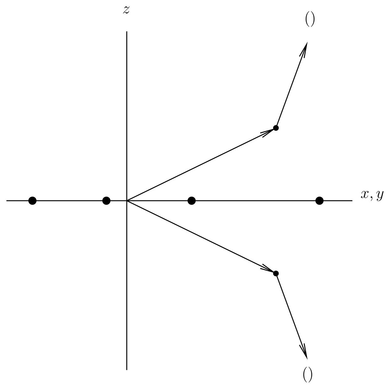
Figure 1:The - plane, viewed from the side. The spots in the - plane are the nuclei. is a typical point, and is the reflection of this point through the - plane. The figure illustrates Eqs. (62) and (63).
From and (60) or (61) it follows that
or
for short. This also follows by inspection of Figure 1.
(a) Every improper rotation can be written as , where is given by (1) and is a proper rotation in axis-angle form. Write
and identify and .
(b) Is a scalar operator? Is a vector operator?
(c) In the electrostatic approximation the Hamiltonian for the electron is
where
Define a unitary operator that acts on the Hilbert space of the electron and that corresponds to above in some reasonable way. I suggest you denote the usual parity operator by , to avoid confusion with the angle . You may find it convenient to refer to different types of rotation operators,
as needed, where .
Work out the conjugation relations,
or simply and for short. Note that for any function ,
The you define should satisfy
If it does not, go back and change the definition so that it does. Notice that since you defined to be unitary, this is equivalent to .
(d) So the system is invariant under reflection in the plane, and we have found an operator corresponding to that reflection that commutes with the electrostatic Hamiltonian . Now we will see if the symmetry persists when we include relativistic corrections.
The spin-orbit Hamiltonian worked out in 25. Fine Structure in Hydrogen and Alkali Atoms{} [see (13)] applies only in the case of a radial electric field. The more general expression [see (49)] is
where the quantity in the square brackets is the sum of an operator and its Hermitian conjugate, to make Hermitian.
Does the operator you defined in part~(c) commute with ? If not, modify it so that it does, and call the new operator . Make sure it is still unitary. Depending on your choice of it is possible that no modification is necessary, then . If , reconsider the commutation relations (68). Also work out the commutation relations
or and for short. Hint: notice that , for all proper rotations and all vectors , , . See Prob. Paragraph.
(e) In quantum mechanics we like Hermitian operators that commute with the Hamiltonian, because they possess simultaneous eigenbases, and for other reasons. The operator you found in part~(d) should be unitary. Find a simple expression for .
Is the you found in part~(d) Hermitian? If not, make a simple modification to it to create a new operator, call it , that is both unitary and Hermitian and that commutes with . If no modification is necessary, then will be the same as obtained in part~(d). If is both unitary and Hermitian, then its its eigenvalues must be . Show that this is so.
Let the electron wave function be
Find the ± components of the wave function , and find the conditions that and must satisfy in order that be an eigenfunction of with eigenvalues .
Thus the Hilbert space breaks up into two orthogonal eigenspaces of , which we denote by , where is the eigenvalue of . Write this as
This system and its symmetry become more interesting when time reversal is added to the mix of symmetries. See the continuation of this problem in Prob. Paragraph.