47. Lorentz Transformations in Special Relativity
Introduction
Before we examine how the Dirac equation and Dirac wave function transform under Lorentz transformations we present some material on the Lorentz transformations themselves. In these notes we will work at the level of classical special relativity, without reference to quantum mechanics, but the presentation is tailored to our needs in the next set of notes when we examine the transformation properties of the Dirac equation. The discussion in these notes is similar to that in 11. Rotations in 3-Dimensional Space, which presented the theory of spatial rotations. Indeed, since spatial rotations are examples of Lorentz transformations, these notes constitute a generalization of 11. Rotations in 3-Dimensional Space in many respects. You may wish to review 11. Rotations in 3-Dimensional Space at this point to orient yourself. You may also wish to look over Appendix E. Introduction to Tensor Analysis for some general information on tensor analysis in special relativity, especially Secs. Lorentz Transformations--The Sign of the Metric, and a Notational Problem. In the following we call on some basic knowledge of special relativity and tensor analysis.
Lorentz Transformations and the Lorentz Group
The usual approach to Lorentz transformations in introductory treatments of special relativity is to work out the transformations that represent boosts, usually following Einstein’s postulate that the speed of light is the same in all reference frames, and then to show that these preserve the Minkowski scalar product shown in (3) below. It is assumed that you are familiar with this approach. Along the way it is sometimes mentioned that ordinary spatial rotations are also Lorentz transformations. In the following we will reverse this sequence of concepts, and define a Lorentz transformation as any linear transformation that satisfies (3). This has the advantage of unifying parity and time reversal with ordinary (proper) Lorentz transformations, which consist of boosts and rotations. In our approach, a general Lorentz transformation is a product of operations that can include rotations, boosts, parity and time reversal.
We begin with a space-time diagram, Figure 1, which shows the coordinate axes of a Lorentz frame as well as a light cone. The light cone has the equation,
It consists of two parts, the forward and backward light cones, the parts and , respectively. The forward light cone is the locus of events generated by a light flash at , that is, by the spherical shell of the light pulse created by the flash, expanding at velocity . The backwards light cone consists of another light pulse in the form of a spherical shell, this one collapsing inward at velocity in such a way that the light reaches the spatial origin at time . As usual in relativity theory, the interior and surface of the forward light cone are the set of events that can be reached from by a signal traveling with velocity , that is, events that lie in the causal future of the event . The interior and surface of the backwards light cone consists of events that can communicate with the event by means of a signal traveling at velocity , that is, events that lie in the causal past of the event .
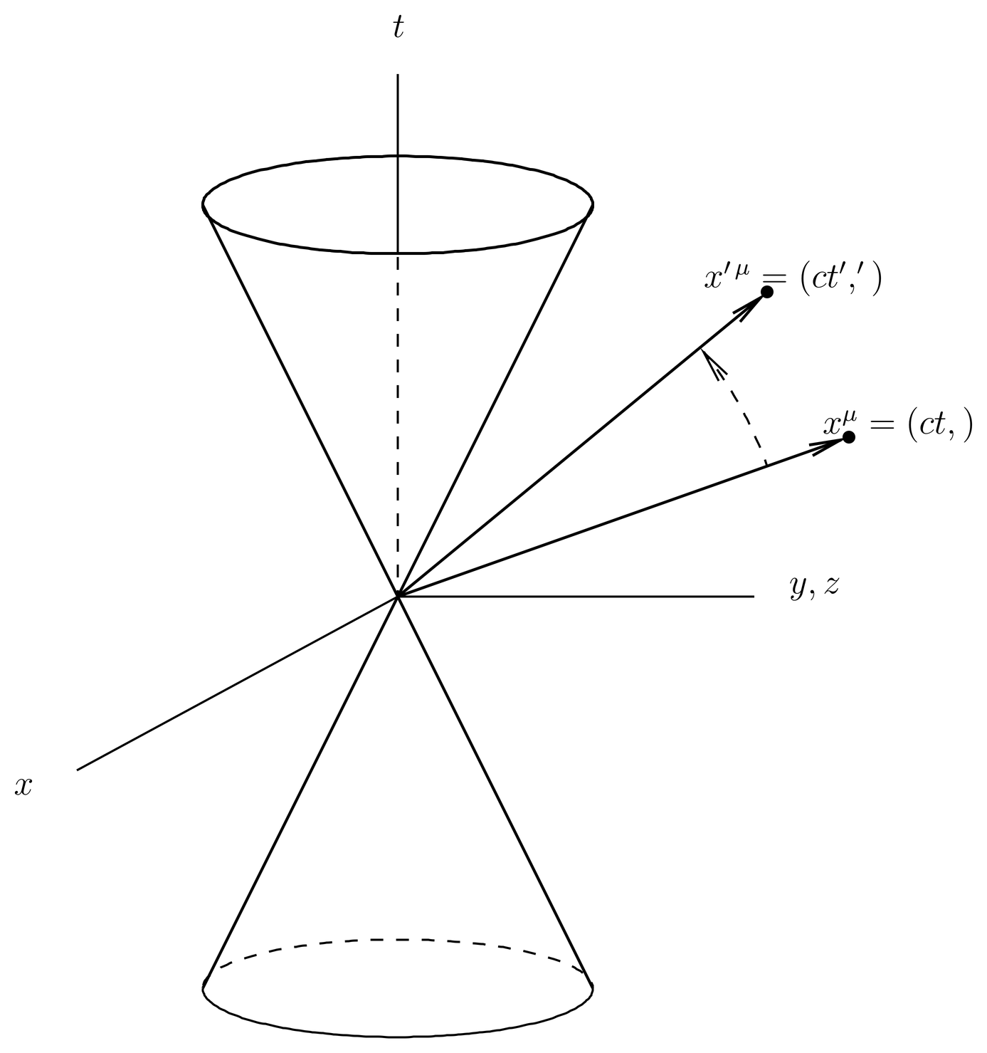
Figure 1:A Lorentz frame with light cone. One of the spatial axes is suppressed to make a drawing possible. Two space time events, and , are shown.
Also shown in the figure is an event with coordinates . We consider a mapping of space-time onto itself, taking the (old) event into a (new) event , as shown. We suppose the mapping is linear and specified by a matrix ,
Only linear transformations map free particle orbits (straight lines at constant velocity) into other free particle orbits. We define the mapping to be a Lorentz transformation if the Minkowski scalar product is preserved, that is, if
for all , where is the Minkowski metric with components
By this definition, the nature of the vector (space-like, time-light or light-like) is preserved by the transformation (3). In particular, the surface of the light cone (the set of light-like events ) is mapped into itself by the transformation, as is the interior (the set of time-like events) and the exterior (the set of space-like events). As we shall see, the interior and surface of the forward light cone may be mapped into itself by the Lorentz transformation, in which case the interior and surface of the backwards light cone is also mapped into itself, or the forward and backward light cones may be mapped into each other, depending on the Lorentz transformation.
Substituting (2) into (3) and juggling indices slightly, we obtain
or, since is arbitrary,
A Lorentz transformation, that is, a matrix specifying a Lorentz transformation, is one that satisfies this equation.
Let us put this into matrix form. Let
in which the first (second) index is understood as the row (column) index. As matrices, and are actually the same [see (76) and (83)], but we shall keep them notationally distinct. Then the condition (6) defining a Lorentz transformation can be written,
where indicates the transpose.
Compare this to the definition of a orthogonal matrix, which can be written
where all matrices are understood to be and where is the identity matrix, representing the Euclidean metric on three-dimensional space. A matrix satisfying this equation is said to belong to , the group of orthogonal matrices. The properties of orthogonal matrices are discussed in 11. Rotations in 3-Dimensional Space. Similarly, (8) shows that a Lorentz transformation can be regarded as a matrix that is orthogonal with respect to the Minkowski metric . A matrix satisfying (8) is said to belong to the group , which indicates the group of matrices orthogonal with respect to a metric with three space-like and one time-like directions. That is, by our definition, is the group of Lorentz transformations.
The proof of the group property works like this. First, note that (now the identity) satisfies (8). Next, by taking determinants of (8), we obtain
since the determinant of the transpose of a matrix is the same as the determinant of the matrix, and since cancels from both sides. This shows that
and, in particular, , so exists. To obtain an expression for we multiply (8) by ,
which shows that
This is not quite as simple as the rule that applies to ordinary orthogonal matrices, but it does make it easy to invert a Lorentz transformation. If (13) is translated into index language, it becomes
Having shown that exists, we now show that it is a Lorentz transformation. We do this by multiplying (8) from the left by , and from the right by . This gives
which shows that is a Lorentz transformation. Finally, if and are two Lorentz transformations, then
which shows that the product is also a Lorentz transformation.
In this discussion and in the rest of these notes on the Dirac equation we view Lorentz transformations as mappings of space-time onto itself, that is, we will take the active point of view. See Active versus Passive Point of View for a discussion of the active and passive points of view. Most introductions to relativity theory take the passive point of view, in which coordinates or tensors are transformed from one coordinate system to another. But we used the active point of view in our development of rotations in quantum mechanics in earlier sets of notes, and for consistency we must continue it with Lorentz transformations. We will give some examples presently of how the active point of view works out in practical examples, as well as some comments about how to think about it.
The Group Manifold of ; Proper and Improper Lorentz Transformations
We now discuss the distinction between proper and improper Lorentz transformations, which is explained geometrically in terms of the group manifold of . You may wish to review Group Manifolds for and , which explains the analogous situation for the group of orthogonal transformations on 3-dimensional space.
The space of Lorentz transformations is 6-dimensional, that is, it takes six parameters to specify a Lorentz transformation. As we shall see, those parameters can be identified with the Euler angles of a rotation and the velocity of a boost. Recall that the space of rotations alone is 3-dimensional, and that it can be parameterized by the three Euler angles. The fact that we need six parameters to specify a Lorentz transformation follows from the definition (8). This equation can be regarded as a constraint that the matrix must satisfy in order to be a Lorentz transformation. In terms of components, there are 10 independent constraints, because both sides of (8) are symmetric, matrices, which have 10 independent components. But a general matrix has 16 components, so the number of independent parameters in a Lorentz transformation is .
The group manifold of can be thought of as the 6-dimensional surface in 16-dimensional matrix space (the space of , real matrices) on which (8) is satisfied. Recall that the group manifold is the 3-dimensional surface in the 9-dimensional space of matrices such that , and that it consists of two disconnected components containing the proper and improper rotations. Recall also that the improper rotations contain the spatial inversion operation represented by the matrix [see (16)].
It turns out that the group manifold consists of four disconnected components, which are distinguished by , which can only take on the values [see (11)], and by the sign of the time-time component of , that is, . The meaning of this component is the following. First of all, it is easy to show from the definition (7) that
Next, in a Lorentz transformation , the 0-th component can be written,
that is, is the coefficient connecting the old time with the new time . This coefficient is the partial derivative,
where it is understood that (the old spatial point) is held fixed in the differentiation. To within a sign, is the relativistic factor of time dilation, given in terms of the velocity of the boost contained in by
If , then as the old time increases, so does the new time, and . In this case the Lorentz transformation maps the forward light cone into the forward light cone, and the backward into the backward. But if , then as the old time increases, the new time decreases. This means that the Lorentz transformation contains a time-reversal operation, and that . In this case the Lorentz transformation maps the forward light cone into the backward light cone and vice versa.
We can exhibit some matrices taken from the four components of the Lorentz group . In the following is the matrix that brings about a spatial inversion but which does nothing to the time:
It is a generalization of the matrix discussed in 11. Rotations in 3-Dimensional Space\ and \parity\ [see (16)]. Also, is the matrix that inverts time but does nothing to the spatial components:
Finally, the matrix inverts all the space-time coordinates:
These matrices appear in Table 1, which gives an example of a matrix taken from each of the four components of . It is easily checked that all four matrices in Table 1 are Lorentz transformations, according to the definition (8).
Table 1:The four components of the Lorentz group are distinguished by and by , which amounts to specifying whether the Lorentz transformation contains a spatial inversion and/or a time-reversal. An example of a matrix taken from each component is shown.
| Matrix | ||
|---|---|---|
| +1 | +1 | |
| -1 | +1 | |
| -1 | -1 | |
| +1 | -1 |
We can picture the group manifold of geometrically as illustrated in Figure 2. The four components are each connected sets that are disconnected from one another. See Fig.~\figr\classrot.4 for the analogous diagram in the case of the group .
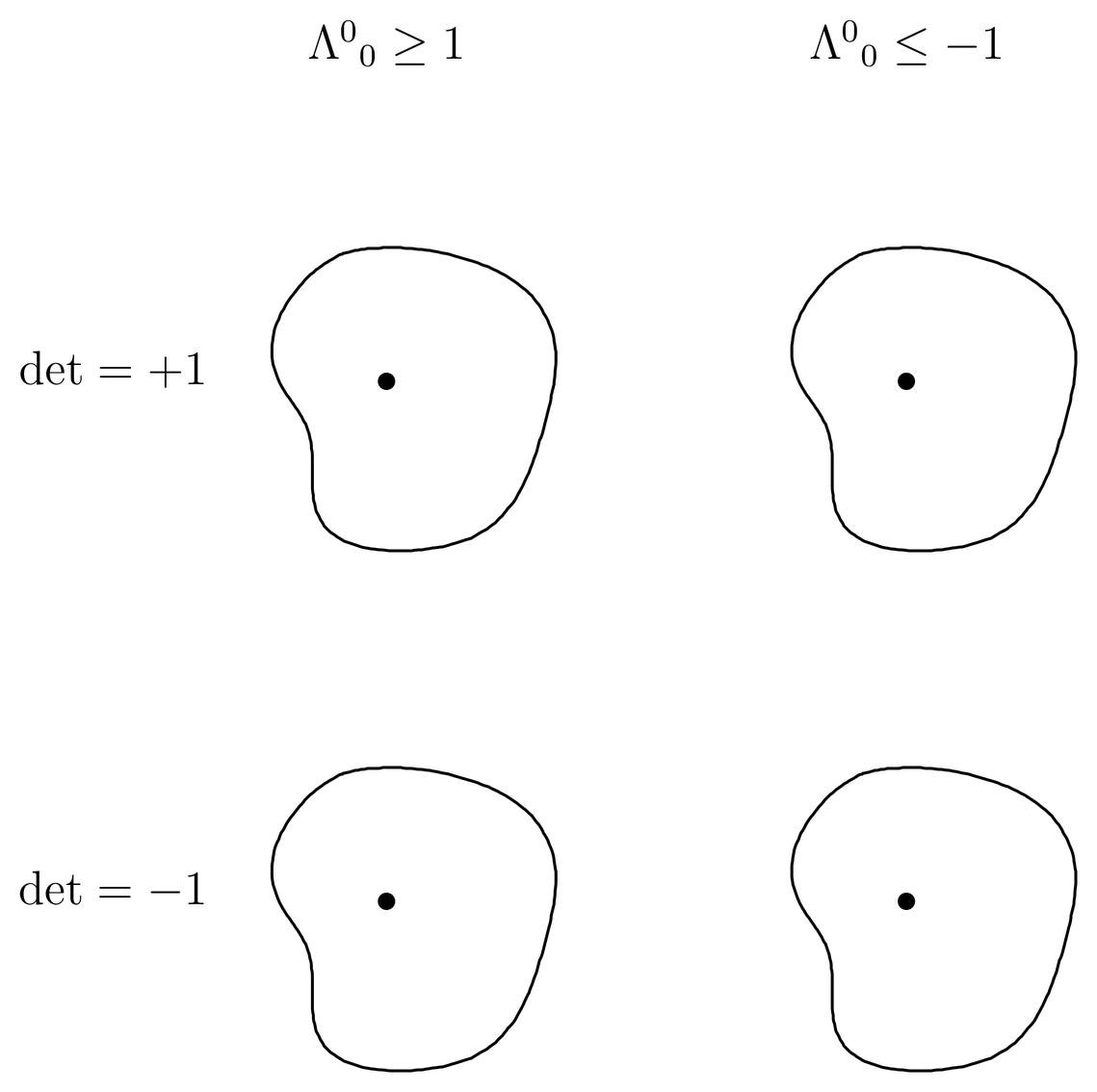
Figure 2:The group manifold of consists of four disconnected components (each component is a connected set, but disconnected from the other components). Each component can be viewed as a 6-dimensional surface inside 16-dimensional matrix space (the space of real, matrices). The four components are distinguished by and by . A sample matrix taken from each component, as in Table Table 1, is illustrated for each component.
The component containing the identity is called the identity component. It consists of Lorentz transformations that can be continuously connected with the identity, that is, transformations that can be built up out of products of infinitesimal Lorentz transformations. We will refer to the Lorentz transformations belonging to the identity component as proper, while all others will be considered improper. The idea is that proper Lorentz transformations consist of proper rotations or boosts, or products of these, but do not contain either a spatial inversion or a time reversal operation. The proper Lorentz transformations constitute a group by themselves, a subgroup of the full Lorentz group .
For the time being we will concentrate on proper Lorentz transformations, and defer a discussion of parity and time-reversal to a subsequent set of notes.
Pure Rotations
Pure rotations are examples of proper Lorentz transformations. They are specified by rotation matrices, which are exactly the same as those presented in 11. Rotations in 3-Dimensional Space, except that now we append a row and column corresponding to the time coordinate, which is not affected by the rotation. As in 11. Rotations in 3-Dimensional Space, we will denote a rotation by angle about axis by . For example, the rotations about the three coordinate axes are
These may be compared to (18). These matrices are interpreted in the active sense, as in 11. Rotations in 3-Dimensional Space, that is, they map an (old) unrotated point to a (new) rotated one.
Pure Boosts
Pure boosts are another example of proper Lorentz transformations. Boosts can be specified by the velocity of the boost, but in the following we shall use a different parameterization, which is convenient for bringing out the analogy with rotations more clearly. First, we define the usual relativistic parameters and in terms of the magnitude of the velocity (a la Jackson, Classical Electrodynamics),
By these definitions and , but sometimes it is convenient to let and take on negative values, so that , where is a unit vector such that is in the same direction as (when ) or opposite the direction of (when ). We call the axis of the boost. With these understandings, , and . Next, it is convenient to introduce the rapidity parameter , defined by
Then the range corresponds to . The rapidity is a kind of hyperbolic angle, which plays the same role for boosts as does for rotations. We will write for the boost along axis with rapidity . The velocity of the boost is given by
We will now work out the explicit form of the matrices . Here we call on some experience with Lorentz transformations in special relativity.
In any boost along a direction , the two spatial coordinates orthogonal to are not affected, while the coordinate and the spatial coordinate parallel to transform according to the matrix,
We interpret this matrix in an active sense. An example will illustrate the meaning of active boosts, as well as showing how the signs in the matrix (28) were determined. Suppose we have a particle of mass at rest. Then its energy-momentum 4-vector [see (19)] is given by
where the 0-subscript means “at rest.” If we multiply the and coordinates of this 4-vector by the matrix (28), keeping the and components fixed, we obtain
which corresponds to the correct energy and momentum for a particle moving down the -axis with velocity . The particle has been boosted with velocity , which is just what we want in the active sense. This allows us to write down the matrix .
Carrying out the same procedure for boosts down the three coordinate axes, we obtain explicit matrices when is one of the coordinate directions. These are
These boosts may be compared to the rotations (24).
We can also obtain an explicit expression for the boost along an arbitrary direction . Let be an arbitrary 4-vector, and let
The boost transforms the time component and the component of the spatial vector along , that is, , according to the matrix (28), while leaving the component of orthogonal to invariant. That is, (32) is equivalent to
Combining the last two equations, we write the overall transformation as
This may be compared to the analogous formula for pure rotations, (44). It may also be compared to Jackson, Classical Electrodynamics, 3rd ed, Eq.~(11.19). The formula in Jackson has minus signs compared to our (34), because he uses the passive interpretation.
A final remark about rapidities is that boosts along the same axis commute with one another, and the rapidities just add when boosts are composed. That is, we have
This may compared with (17), which shows the analogous property for rotations. We note that boosts along different axes do not commute, in general.
Property (35) may be proved by composing two transformations of the form (34), but since the coordinates orthogonal to the direction of a boost are not affected by the boost, the essence of the proof is just the multiplication of matrices of the form (28). In fact, calling that matrix , it is easily verified that
Rapidities and velocities are related by
so the velocity that results on composing two boosts with rapidities and along the same axis is
where we use the addition formula for the function. But this is equivalent to the usual rule in special relativity for composing velocities,
This rule has the property that if and , then . It is equivalent to the statement for all .
A Useful Theorem, and Parameters of Proper Lorentz Transformations
We have presented boosts and rotations as examples of proper rotations, but there is a theorem that states that every proper Lorentz transformation can be factored in a unique way into the product of a rotation times a boost,
where has some axis and angle , and where has some axis and rapidity . We will not prove this theorem (the proof is accomplished most easily in terms of the spinor representations of the proper Lorentz group), but it is a useful fact. It shows in particular that the six parameters specifying an arbitrary proper Lorentz transformation can be taken to be the three inherent in (or, equivalently, the three Euler angles), plus the three inherent in (or, equivalently, the velocity ).
Exponential Notation for Rotations and Boosts
It was shown in 11. Rotations in 3-Dimensional Space\ that proper rotations can be written in exponential form,
[see (40)]. Here is a “vector” of matrices, given by
These are the same as the matrices (22), except that we have appended a row and column of zeroes to take care of the time component. That is, these matrices have a block diagonal structure, where the lower block is the same as in (22).
Boosts can also be represented in exponential form. First we consider an infinitesimal boost, in which . Notice that when is small, then , which gives a physical interpretation to the rapidity in this case. Specializing (34) to the case of small and neglecting terms of order , we have
where are the spatial components of . This can also be written,
where is another “vector” of matrices, given explicitly by
(44) is the form of an infinitesimal boost, which may be compared to (32), which applies to infinitesimal rotations.
Now following the logic of Exponential Form of Finite Rotations, starting with (42), we can obtain an exponential form for boosts when is not small. If is not small then we can use (35) to write
where we can choose large enough to make as small as we like. This makes it plausible that
which by the limit discussed in Exponential Form of Finite Rotations gives
This is the exponential form of boosts, which may be compared to (41) for rotations.
Infinitesimal Lorentz Transformations
Infinitesimal rotations were studied in 11. Rotations in 3-Dimensional Space; when the angle is small, then
[see (32)]. This can be regarded as the first two terms of the exponential series in (41). Similarly, (44) gives the form of infinitesimal boosts, which can be regarded as the first two terms of the exponential series in (48). Now multiplying the infinitesimal rotation (49) by the infinitesimal boost (44) and using the theorem (40), we obtain a general, proper, infinitesimal Lorentz transformation,
where we have neglected terms that are second order in the small corrections. We see that an infinitesimal Lorentz transformation is the identity plus a correction matrix that is a linear combination of the six matrices , , .
These six matrices constitute the Lie algebra of the Lorentz group. They satisfy commutation relations that can be worked out directly from the definitions (42) and (45),
The first of these commutators was already given in (34), and we have seen that it is a classical version of the standard angular momentum commutation relations in quantum mechanics, as explained in 13. Representations of the Angular Momentum Operators and Rotations. The second of these equations is a classical statement of the fact that transforms as a vector under rotations [see (21) for the definition of a vector operator in quantum mechanics]. The third of these commutation relations shows that rotations can be generated as products of pure boosts. For example, when is small, the Lorentz transformation
is a pure rotation about the -axis. See the discussion in The Noncommutativity of Rotations. The fact that pure rotations can be generated by products of noncommuting pure boosts lies behind Thomas precession, an effective rotation that is experienced by accelerated frames. Thomas precession is responsible for canceling one half of the spin precession expected due to spin-orbit coupling. See the discussion in The Hamiltonian.
A Covariant Approach to Infinitesimal Lorentz Transformations
Infinitesimal Lorentz transformations are important because an arbitrary, proper Lorentz transformation can be built up as products of them. But the decomposition of them into rotations and boosts, as in (50), is not entirely covariant. That is, what is purely a boost in one frame is partly a boost, partly a rotation in another. We now develop a completely covariant approach to infinitesimal Lorentz transformations (that is, to the Lie algebra of the group), which will be useful to us in 48. Covariance of the Dirac Equation{} for establishing the covariance of the Dirac equation. (Note that the words “covariance” and “covariant” have two distinct meanings, as explained in Introduction.)
Let a Lorentz transformation have the form,
where is the correction matrix and is a small scale factor used to remind us that the correction is small. This Lorentz transformation is infinitesimal. Plugging this into the definition (8) of a Lorentz transformation, we have
or, through first order in ,
This shows that is an antisymmetric, matrix. Compare this to what we did with ordinary rotations in Infinitesimal Rotations.
As in Infinitesimal Rotations, it is convenient to introduce a basis of antisymmetric matrices. The difference is that now we are dealing with matrices, so the basis consists of six matrices altogether. Let be the matrix with a 1 in component and a -1 in component (the just stands for “antisymmetric”). The indices attached to are labels of the matrix, not component indices. If we wish to specify the components of the matrix , we will write . According to the definition, these components are
where the two terms put a 1 in slot , and a -1 in slot . The matrices satisfy
in particular, they are antisymmetric. If we let and run over , we get 16 matrices altogether. We can think of these matrices as constituting an antisymmetric, “tensor” of antisymmetric matrices, much as constitutes a “vector” of matrices. Since this “tensor” is antisymmetric, that is, , four of these matrices vanish and the remaining twelve consist of six pairs that are equal and opposite. We see that there are only six linearly independent matrices , which we get by restricting and to the range .
Thus a given antisymmetric matrix, such as in (55), can be written as a linear combination of the six independent matrices with coefficients that we will call :
In this equation, you must remember that are numbers and are matrices. Given , the numbers are uniquely determined for . We now define for other values of , by requiring,
so that can be thought of as an antisymmetric, matrix or space-time tensor. Then using (57), the expansion (58) can be written,
where we drop the sum and use the summation convention, since now we have an unrestricted sum over and .
Finally, we multiply (60) by and write the result as
where
Again, the indices , on are labels of the matrices, not component indices. You may compare (61), the expansion of the correction matrix for an infinitesimal Lorentz transformation in terms of a set of basis matrices, with (21), the analogous expression for pure rotations.
Combining (53) and (61), we can write the infinitesimal Lorentz transformation itself as
where we have absorbed the into the parameters , which, as noted, are small. Since both this expression and (50) represent general, infinitesimal Lorentz transformations, they must be equal to each other.
To establish the connection between these two expressions, we first work out the components of , which, according to (7) and (62), are the same as the components of with the first index raised. The components of are given by (56). Raising the index in that equation, we obtain
If we set or in this expression and work out the components of the matrices, we find
where and are given by (42) and (45). Thus, the antisymmetric “tensor” of matrices is equivalent to the two “vectors” of matrices and , and it contains the Lie algebra of the Lorentz group. The commutation relations (51), expressed in terms of the matrices , , can be expressed in terms of the matrices . Alternatively, the commutation relations among the can be worked out directly from (64). Although we will not use the result we note it for reference:
Breaking the sum on , in (63) into its space and time components and using (65), we can write the infinitesimal Lorentz transformation as
Comparing this to (50), we can read off the relations between the six parameters , , and of an infinitesimal Lorentz transformation, and the six independent parameters contained in . To do this it is convenient to define two vectors,
and
which are equivalent to
and
Then these vectors are related to the coefficients by
and
If the infinitesimal Lorentz transformation is a pure rotation, then
and
If the infinitesimal Lorentz transformation is a pure boost, then
and
Active and Passive Lorentz Transformations
In Pure Boosts we made a few comments about how to interpret Lorentz transformations in an active sense. Here we will elaborate somewhat on this question. We mainly think in terms of boosts, since the active interpretation of rotations was covered in 11. Rotations in 3-Dimensional Space.
Let the world line of a particle be given by , where is the proper time. Then under an active, proper Lorentz transformation specified by matrix , the state of motion of the particle specified by mapped into a new state of motion , given by
In Pure Boosts we considered the special case in which the original motion was that of a particle at rest, but here can represent any state of motion, including accelerated motion. The momentum transforms by the same matrix as the space-time vector , since
See (49). Notice that is invariant under proper Lorentz transformations.
In the passive point of view which is used in most introductions to special relativity one speaks of two frames, the “lab” and “moving” frames, and one studies the relation between the space-time coordinates of the particle as seen in the two frames. To connect the present, active interpretation with the passive interpretation, first consider boosting a particle with space time coordinates in the active sense. Let the Lorentz transformation be parameterized by the velocity of the boost, so that the space-time coordinates of the particle after the boost are
where we put an subscript on to indicate that it is the velocity of the boost in the active interpretation. The meaning of is that if we boost a particle at rest, then is the velocity of the particle after the boost.
To obtain the passive interpretation we need a second frame. To obtain it we boost not only the particle but also the original Lorentz frame, both by the same Lorentz transformation . This produces a boosted frame, the velocity of which with respect to the original frame is . Also, the space-time coordinates of the particle with respect to the boosted frame are the same as the space-time coordinates of the original particle with respect to the original frame, that is, they are in (80). Now we interpret the boosted frame as the “lab” frame and the original frame as the “moving” frame. Then (80) can be written,
However, in the passive interpretation we usually parameterize the boost by the velocity of the moving frame with respect to the lab frame, which is in the present notation.
In summary, the active equation (80) is put into passive form by interpreting as and as , and changing the sign on the velocity parameter of the boost. You may compare our (34) with Jackson’s Eq.~(11.19) with this rule in mind.
Transforming Fields
(78) gives the rule for Lorentz transforming the state of a particle in an active sense, but how do we transform fields? For example, what does it mean to boost a field? The answer can be given in a physical sense, for example, in the case of the electromagnetic field . The electromagnetic field is produced by charges and currents, according to the Maxwell equations,
where is the electric current 4-vector. The current in turn is produced by charges in some state of motion. It is logical to define the Lorentz transformed current as the current produced by the charges in the Lorentz transformed state of motion, according to (78), and the Lorentz transformed electromagnetic field as the field produced by the Lorentz transformed current. See Problem~\prbrlorentz-2 where these ideas are explored.
The same results can be obtained in another way. Let us begin with the example of a scalar field on 3-dimensional space. If we apply an active rotation specified by a matrix , then it is logical to define the rotated field as the one that we get by allowing the points to carry the value of the scalar field with them as they are rotated. That is, if is an “old” point and is a “new” or rotated point, then we require that the rotated field satisfy
In words, the value of the new field at the new point is equal to the value of the old field at the old point. This same rule was discussed in \orbamsph.2 in connection with the transformation properties of the wave function of a spinless particle, see (15). Although that discussion was framed in terms of the transformation of a quantum wave function, the same concepts apply to any scalar field, for example, the temperature or pressure of a fluid. If we substitute into (83) we get
or, making the replacement ,
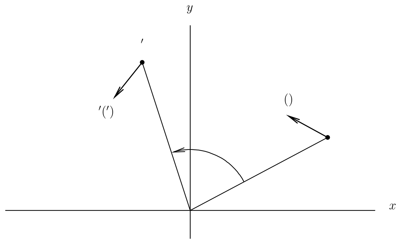
Figure 3:When we rotate a vector field such as an electric field, we rotate the value of the field along with the point at which the field is evaluated.
What about a vector field, such as an electric field ? The most obvious definition of the rotated field from a geometrical standpoint is illustrated in Figure 3, in which the value of the field is rotated along with the point at which the field is evaluated. That is, the rule is
where again . Again making the replacement , this becomes
Now let be a scalar field on space-time, where stands for all four space-time coordinates or . The transformation law (85) for scalar fields under ordinary rotations suggests that scalar fields should transform under Lorentz transformations according to
Examples of scalar fields in electromagnetism include
and
the two classic invariants of the electromagnetic field. [Actually, the quantity (90) is a pseudo-scalar, not a scalar.] Another scalar field is the Klein-Gordon wave function studied in 45. Introduction to Relativistic Quantum Mechanics and the Klein-Gordon Equation.
Similarly, let be a vector field on space-time. Then the transformation law (87) for vector fields under ordinary rotations suggests that vector fields should transform under Lorentz transformations according to
Indeed, it is shown in Prob.~\prbrlorentz-2 that the electric current transforms in exactly this way, when the particles creating the current are boosted by . Similarly, the electromagnetic field tensor transforms according to
In the next set of notes we will consider how Dirac spinors transform under Lorentz transformations, a necessary step in discussing the covariance of the Dirac equation.
Problems
Problem 1.
Some general properties of Lorentz transformations, following from the definition (\eqr\cn.6) or (\eqr\cn.8).
(a) Show that if a matrix satisfies (8), then the component satisfies (17). Hint: Examine the 00 component of (8).
(b) Below (19) we referred to “the velocity of the boost contained in .” In this part of the problem we will explain what this phrase means. Let a particle have a world line specified by , where is the proper time, that is, the time as indicated by a clock carried by the particle. We allow the particle to be in any state of motion, in particular, the particle may be accelerated. When we apply a Lorentz transformation specified by to this particle, interpreted in the active sense, we obtain the same particle in a different state of motion specified by , where
The proper time is the same before and after the Lorentz transformation, because
This implies that is invariant.
Now suppose the particle is at rest before the Lorentz transformation is applied. Express the four components as explicit functions of . Let be the velocity of the particle after the Lorentz transformation, and express its components in terms of and . We regard this as the velocity of the boost contained in . Use this expression to prove (20).
Problem 2.
Boosting particles to get the boosted current. In this problem we choose units so that .
(a) Consider a particle of charge whose trajectory through space is given by . Let be a field point. Then the charge and current densities are
where is the velocity of the particle.
Now let be the proper time of the particle as measured by a clock carried along with the particle. Also let the proper time and the coordinate time be related by a function ,
and let
This is a way of expressing the 4-vector giving the space-time coordinates of the particle as a function of the proper time,
Show that the current 4-vector is given by an integral along the particle’s orbit (and remember that ),
where if is a 4-vector then
Hint: Use the -integration to eliminate the delta function .
(b) If the particle motion is mapped into a new motion by a Lorentz transformation ,
then show that the 4-current produced by the Lorentz transformed particles is given by
Hint: Use the fact that if is a matrix and is a 4-vector, then
Problem 3.
Let and be two 4-vectors. Let us write
as a shorthand for the Minkowski scalar product. Let be a shorthand for the 4-vector whose -th component is . Show that