12. Rotations in Quantum Mechanics, and Rotations of Spin-1/2 Systems
Introduction
In these notes we develop a general strategy for finding unitary operators to represent rotations in quantum mechanics, and we work through the specific case of rotations in spin- systems. We find that the relation between spin- rotations and classical rotations is two-to-one, due to the appearance of non-classical phase factors. In a certain sense spin- rotations constitute a basic building block in the theory of rotations in quantum mechanics, out of which rotations for an arbitrary system can be constructed. The general theory of rotations in quantum mechanics will be developed in later sets of notes.
Physical Meaning of Rotations in Quantum Mechanics
In classical mechanics, we can rotate the state of a dynamical system, that is, we can rotate all the position and velocity vectors for each particle, to create a new or rotated state. Similarly, in quantum mechanics, given a state (taken for simplicity to be pure), it is possible to define a rotated state such that the expectation values of all vector operators in the rotated state are rotated relative to the expectation values in the original state, exactly as classical vectors would transform under rotations in a classical system. The transformation between the original quantum state and the rotated quantum state is brought about by means of a certain rotation operator, which is unitary because probabilities must be preserved under rotations.
What does it mean physically to rotate a quantum state? Certainly we cannot go in with a wrench, and rotate the wave function of the electrons in an atom, or rotate the spins of those electrons. In any case, as we have emphasized, the wave function represents the properties of an ensemble of systems, not an individual system, so rotating a quantum state must be equivalent to rotating the properties of the ensemble. One point of view is to identify a quantum state with the apparatus that prepares the ensemble of systems about which the quantum state makes statistical predictions. We can certainly rotate a preparation apparatus, and it is logical to regard the state prepared by the rotated apparatus as the rotated state. This point of view gives us a definition of a rotated state, without however specifying the phase of that state.
Alternatively, quantum systems may experience rotations as a result of their time evolution. For example, many small molecules are approximately rigid bodies, and their time evolution is approximately given by a time-dependent rotation operator, just as the time evolution of a classical rigid body is specified by a time-dependent rotation (see Group Manifolds for and ). For another example, spins in magnetic fields evolve by means of a time-dependent rotation operator. The magnetic field can either be external or internal; for example, the electrons in an atom precess in the magnetic field of the nucleus (which is a moving charge in the electron rest frame, and which may have an intrinsic magnetic field of its own). Or the magnetic field may be external, permitting experimental control over the orientation of spins. Another example of rotations in quantum mechanics is produced by Thomas precession, a relativistic but purely inertial effect that rotates all the dynamical variables of an accelerated system, for example, the spin of an electron in an orbit in an atom. Different subsystems of a given system may be rotated by different amounts, for example, it is possible to change the orientation of a molecule without rotating its spins (hit it with another molecule), or vice versa (apply a magnetic field). Thus we speak of spatial rotation operators, spin rotation operators, etc.
The phases associated with rotations are observable. For example, in a neutron interferometer, it is possible to split a beam of neutrons into two, and to subject one of the two resulting beams to a magnetic field, which will rotate the neutron spins. By recombining the beams and observing the interference pattern, phase shifts such as the -1 multiplicative factor that occurs on rotating a spin- system by can be observed. This is a rather direct observation of a phase shift, but phases also enter into quantization conditions (recall the Bohr-Sommerfeld rules), and theoretical predictions of energy levels would not agree with experiment if all phases were not accounted for correctly.
Postulates for Rotation Operators
Suppose we have some quantum mechanical system, and an associated Hilbert space of states. We will be interested in finding operators that act on these states that represent the action of rotations at the classical level. If a classical rotation is specified by a rotation matrix (relative to some inertial frame), then we will denote the associated operator by . For the time being we will work only with proper rotations, so that . We will denote the association itself by
which simply means that is a function of the classical rotation .
As you might imagine, the specific form of the operators depends on the system, but it turns out that there is a great deal that can be said about these operators without going into the specific nature of the system. These are the properties of rotation operators that follow from the properties of classical rotations, that is, ultimately from the Euclidean geometry of three-dimensional space. We will concentrate on these properties first, and then deal with specific physical systems (spin systems, central force problems, atoms, etc) which are treated in later sets of notes.
We make a series of reasonable assumptions or postulates that the rotation operators should satisfy. First, these operators should be unitary, because a symmetry operation should preserve probabilities:
Next, we assume that when the classical rotation is the identity, so is the unitary operator,
Finally, we assume that the unitary operator corresponding to the product of two rotations is the product of the unitary operators, so that
This means that the unitary operators reproduce the multiplication law of classical rotations. These requirements imply that inverse rotations are mapped into inverse unitary operators,
If the requirements (2) to (5) are satisfied, then we say that (more precisely, the mapping (1)) forms a representation of by means of unitary operators. As we will see, these requirements are actually too strong, and in the case of systems of half-integral spin, they cannot be met; for such systems we can almost find a representation, but we ultimately fail because of phase factors. However, the search for a unitary representation of the classical rotations is educational, and the phase factors are not so much a difficulty as an opportunity for obtaining a deeper understanding of rotations, and for finding new physics at the quantum level.
In addition to the mathematical requirements given by (3) to (5), the operators must also satisfy physical properties we expect of rotations. For example, the expectation values of vector operators should transform as classical vectors.
Representations of Near-Identity Rotations
The key to finding a unitary representation of the rotations is to begin with near-identity rotations. First, some notation. We notice that a rotation in axis-angle form actually depends only on the product of the axis and the angle,
so we introduce a vector of angles defined by
and write for the rotation. Now if the rotation is near-identity, we can approximate it by the leading terms of the exponential series,
which is (32). This implies that
for .
The unitary operator that corresponds to the rotation can also be parameterized by , so we will write . In the case of small angles, we can approximate by the leading terms of its Taylor series,
where the first term is 1 (the identity operator) because of (3). At this point you may wish to review the manner in which we defined linear momentum as the generator of translations in 04. Spatial Degrees of Freedom, or the manner in which we defined the Hamiltonian in 05. Time Evolution in Quantum Mechanics. See especially (34), (70), (6) and (8). Following the pattern of those definitions, we now define the angular momentum of the quantum system as the vector operator with components given by
This defines relative to some definition for the unitary rotation operators , so different systems, with different definitions of rotation operators, will have different definitions of the angular momentum (for some it will be orbital angular momentum, for others,spin, etc). This definition of angular momentum allows us to write a near-identity rotation as
We split off a factor of in the definition of in (11) so that the operators will be Hermitian, because in quantum mechanics we think of Hermitian operators as the generators of unitary operators. The Hermiticity of follows by substituting (12) into (exactly as we proved the Hermiticity of the operator in The Generator of Translations). As for the factor of , it makes have dimensions of angular momentum.
Reverting now to our original axis-angle notation, we can write the near-identity rotation operator as
Since the operators were defined in terms of , this is not an explicit solution for the rotation operators , even for infinitesimal rotations. But at least is shows how those rotation operators depend on the axis and angle, which is progress. Note that is a fixed set of three Hermitian operators that are independent of the axis or angle. In a moment we will extend this relation to arbitrary angles.
When defining the angular momentum in quantum mechanics, we have some of the same issues we faced earlier when trying to define linear momentum in quantum mechanics by taking over some definition from classical mechanics. In the case of linear momentum, we decided that the role that linear momentum plays in classical mechanics as the generator of translations was the most fundamental role; this supersedes definitions such as , which are not as general. Similarly, in quantum mechanics, we will define the angular momentum as the generator of rotations, rather than as , which is not as general. For not only is meaningless for systems such as spin systems, but even for the spatial degrees of freedom of a spinless particle, it is not always true that the generator of rotations is (for example, in the presence of magnetic fields). We take the generator of rotations to be the most fundamental role of angular momentum, because, among other reasons, these generators (the components of ) are conserved in systems with rotational symmetry. Moreover, the generality of our definition allows us to treat the angular momentum of orbital motion, spin systems, systems in magnetic fields, multiparticle systems, relativisitic systems and quantum fields under the same formalism.
Rotation Operators for Any Angle
The relation (13), which gives when is small, can be extended to a closed formula valid for any . The pattern follows what we did earlier with translation operators in The Generator of Translations and with classical rotations in Exponential Form of Finite Rotations. We begin by seeking a differential equation for . By the definition of the derivative,
But since the operators form a representation of the classical rotations [see (4)] and since rotations about a fixed axis commute [see (17)], we have
and the numerator in (14) has a common factor of that can be taken out to the right. Thus we have
The remaining limit can be evaluated in terms of the angular momentum with the aid of (13), where the small angle of that formula is identified with here. This gives the differential equation,
Subject to the initial condition , this has the unique solution,
This solution can also be obtained as the limit of the product of a large number of small angle rotations, as in Exponential Form of Finite Rotations [see (42)--(43)].
(18) shows that we can find the rotation operators corresponding to the classical rotations once we know the angular momentum operators . This greatly simplifies the problem, because there are only three angular momentum operators, but an infinite family of rotation operators. The angular momentum operators are not arbitrary, however; in addition to being Hermitian, they must satisfy certain commutation relations.
Commutation Relations for Angular Momentum
Let us consider the rotation defined in (65), and its unitary representative . We have
Let us expand both sides of this equation in a Taylor series in the angles and , defined by and . The answer can be obtained in two ways. In one approach, we expand the exponentials for , , etc., according to (18), and multiply the series. This gives
The calculation is similar to that in (66) leading to (67). When the series are multiplied, first order terms vanish, but at second order the product becomes
On the other hand, according to (68), is a near-identity rotation with axis and angle , , where and are given by (69). Therefore
where we use (69). This is consistent with (21) only if
By setting and to , , , we obtain
These are the standard commutation relations for angular momentum in quantum mechanics, here extracted from the properties of rotation operators. These commutation relations are the quantum analogs of the classical commutation relations (34) for the matrices; the two commutation relations are the same, apart from conventional factors of and .
The usual approach to deriving the angular momentum commutation relations (24) in elementary courses in quantum mechanics is to work with the specific example of orbital angular momentum, whose definition is taken over from classical mechanics. One then just works out the commutators of the components of , and argues that other forms of angular momentum such as spin ought to have the same commutation relations. Here we have derived the angular momentum commutation relations in all generality, following from the properties of rotations. The specific case of orbital angular momentum will be dealt with in 15. Orbital Angular Momentum and Spherical Harmonics.
We have shown that the only way the unitary operators can reproduce the multiplication law for the classical rotations is if the infinitesimal generators in each case satisfy the same commutation relations, apart from conventional factors of and . Therefore we adopt the following strategy in developing the general theory of the representations of classical rotations. We begin by seeking the most general form that a vector of Hermitian operators can take, given that it satisfies the commutation relations (24). For example, we will be interested in the matrices that represent these operators in some appropriately chosen basis. When we have found specific operators that satisfy the commutation relations (24), we will say that we have found a representation of those commutation relations. Next, given some such operators , we exponentiate linear combinations of them as in (18), to obtain the unitary rotation operators . These can also be represented as matrices in some basis. Finally, we explore the physical implications of these operators, to guarantee that they have the physical properties we expect of rotations.
Angular Momentum and Rotation Operators for Spin- Systems
Thus, we must begin by finding a representation of the angular momentum commutation relations (24). We will take up the general problem of doing this in 13. Representations of the Angular Momentum Operators and Rotations; for the remainder of these notes, however, we will restrict consideration to a spin- system, which possesses a 2-dimensional ket space. To find operators acting on this space that satisfy the commutation relations (24), we simply notice that
will do the trick. This is because of the commutation relations for the Pauli matrices,
Therefore we provisionally take the rotation operators to be
where we use the standard properties of the Pauli matrices to reexpress the Taylor series for the exponential in terms of trigonometric functions (see Prob. Paragraph).
The identification of the operators with rotations is provisional because we must show that these operators make physical sense as rotations. For example, let us consider the Stern-Gerlach experiment, in which we measure the components of the magnetic moment vector . We showed earlier that the operators corresponding to the components of , when represented in an eigenbasis of with appropriate phase conventions, produce matrices proportional to the Pauli matrices . Therefore, since we expect transform as a vector under rotations, so should . This means that if we have an (old) state , and a new or rotated state , then we expect that the expectation values of in the old and new states should be related by the classical rotation . In other words, we should have
or, since this must hold for all ,
where it is understood that and . In case (29) it not clear, we write it out in components,
To see if (29) is true, we simply substitute (27) to obtain
Next we use the properties of the Pauli matrices to derive the identities,
which we use to rewrite (32) in the form,
Finally, by comparing this with (44), we see that (29) is verified. Encouraged by this result, we henceforth consider the operators defined by (27) to be rotation operators for spin- systems.
The Spin- Adjoint Formula
Before leaving the result (29), however, we will comment on it further, since it is useful in its own right. In fact, this result is a spinor version of the adjoint formula (48), which we derived earlier for classical rotations. To see the analogy more clearly, we first replace by and by in (29), so that
Next we dot both sides by some vector , and use (74) to obtain
This may be compared to the adjoint formula (48) for classical rotations, which we reproduce here with a slight change of notation:
We will refer to (35) or its variants as the adjoint formula for spinor rotations.
The Double-Valued Representation
We seem to be in good shape for the interpretation of the operators as spinor rotations. There is, however, one wrinkle, which we find upon looking at specific examples of rotations. In particular, if we rotate a spinor about some axis by the angles of and , we find
according to (27). We see that the spinor of an electron or other spin- particle rotated by does not return to its original value, but rather undergoes a phase change of -1.
The fact that a rotation is not the identity operation is a nonclassical effect, and we must first ask what the physical significance is (in particular, whether it has any physical consequences). Certainly an overall phase factor of a quantum state has no physical significance, but it is possible to split a beam of spin- particles into two, and to subject one of the resulting beams to a rotation by , whereupon the phase shift becomes observable in the interference pattern that results when the beams are recombined. This experiment has actually been performed with neutron beams, which are split and recombined by means of a neutron interferometer (essentially a large silicon crystal used as a kind of neutron diffraction grating). These experiments are discussed in more detail by Sakurai, Modern Quantum Mechanics, and they show that we must take the -1 phase shift for rotations to be real.
The fact that a rotation is not the identity operation on spinors of spin- systems means that we must reconsider our original quest for a representation of the classical rotations by means of unitary operators acting on a ket space, as laid out by (1)--(5). In fact, the operators defined by (27) do not form a representation of the classical rotations in the strict sense of the word, simply because they are not parameterized by the classical rotations. That is, the operators are not a function of the matrices, at least not in the sense of a single-valued function; this is clear from the special case of
a single classical rotation for which there are two unitary operators, shown by (38). More generally, it can be shown that corresponding to every classical rotation there are two unitary spinor rotations,
which replaces (1). The two unitary operators corresponding to a given differ by a sign. We see that the association between classical and spinor rotations is not one-to-one, but rather one-to-two.
In view of this, notation such as is not really proper for spin- rotations, without some understanding as to which of the two unitary operators is meant. [On the other hand, the notation is unambiguous, as indicated by (27).] For example, the representation law (4) could be rewritten in the form,
which would mean that if we take one of the two unitary operators corresponding to and and multiply them, we will obtain one of the two unitary operators corresponding to . With this interpretation, (41) is correct for spinor rotations (but it is awkward and can lead to confusion).
The Group Manifolds and 
We explained in 11. Rotations in 3-Dimensional Space\ that the Baker-Campbell-Hausdorff theorem guaranteed that the group composition or multiplication law for finite operations was effectively contained in the commutation relations. This was why we focused first on finding a representation of the commutation relations (24), a task that will occupy us at greater length in the next set of notes, and why we were confident that when we exponentiated linear combinations of the angular momentum operators we would obtain operators that would reproduce the composition law of the classical rotations. What, then, has gone wrong, that we should end up with a double-valued representation, so that (4) must be replaced by (41)? The answer is that the spinor representation of the rotations is locally one-to-one, but globally one-to-two.
To explain this statement more precisely, we need to discuss the group . The notation is standard in mathematical physics for the group of complex unitary matrices with determinant +1. As in the notation , the stands for “special,” which means the determinant is +1.
The significance of in the present discussion is that every spinor rotation defined by (27) for some axis and some angle is a member of the group ; and, conversely, every member of the group can be written in the form for some axis and some angle . We will not prove these facts; the proofs are easy, and are left as exercises. But we note the following consequence. Namely, since any group is closed under multiplication, if we form the product of two spinor rotations of the form , we obtain another spinor rotation of the same form. Thus, every spinor rotation can be written in axis-angle form, and (like the classical rotations) there is no loss of generality in assuming this form for a spinor rotation. We see that is the group of spinor rotations.
To understand the one-to-two association between and more thoroughly, it helps to view things geometrically in terms of the respective group manifolds. As explained in 11. Rotations in 3-Dimensional Space, the group manifold for can be seen as a 3-dimensional surface living in the 9-dimensional space of all real matrices. Similarly, the group manifold for can be seen as a surface living in the space of all complex matrices. Since a complex matrix has 4 complex components, each with a real and imaginary part, it takes 8 real numbers to specify an arbitrary complex matrix, and we can say that complex matrix space is 8-dimensional. But the condition constitutes 4 real constraints, and the condition is one more real constraint, for a total of 5 constraints on 8 variables. Therefore the group manifold can be seen as a 3-dimensional surface living in the 8-dimensional space of all complex matrices. We see that both group manifolds and are 3-dimensional; this is also evident from the axis-angle parameterization of matrices, which involves 3 real parameters.
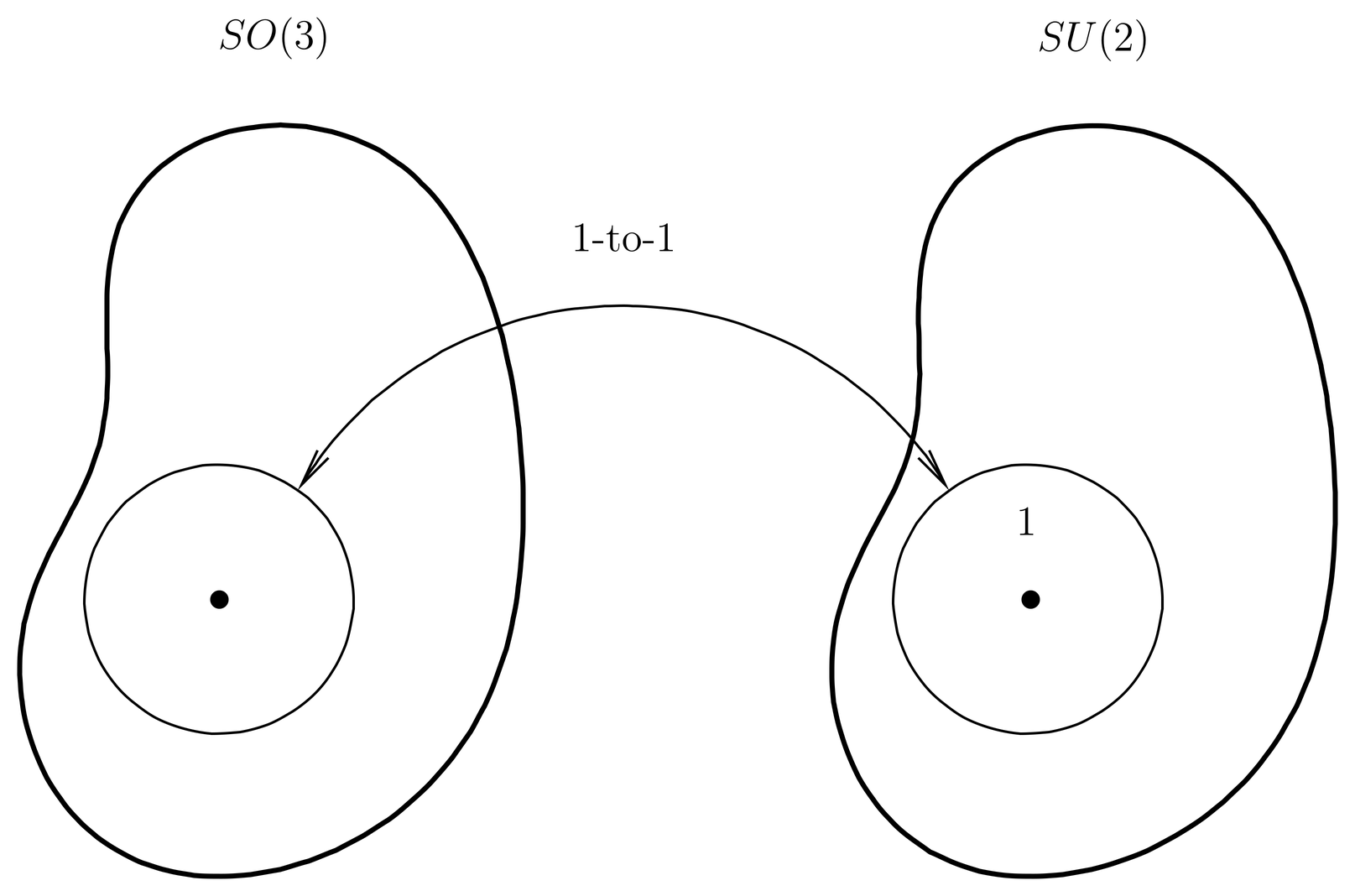
Figure 1:There exist finite neighborhoods of the identity elements in the two groups, and , which can be placed into one-to-one correspondence in such as way that the composition law is reproduced, according to Eq. (4). But the neighborhoods cannot be expanded to cover the whole group manifold without losing the one-to-one correspondence.
The identity matrix is one point of interest on the group manifold , and the identity is one point of interest on the group manifold . These two points are associated with one another by the requirement (3). Next, once we have found a representation of the angular momentum commutation relations by (25), we have a one-to-one correspondence between infinitesimal neighborhoods of the respective identity elements, as indicated by (13). Next, the Baker-Campbell-Hausdorff theorem guarantees that by exponentiation we obtain a one-to-one correspondence between finite neighborhoods of the identity elements, which moreover satisfies the representation law (4). This is illustrated in Figure 1, and it is in this sense that we say that the representation of by is locally one-to-one. But if we try to expand the two neighborhoods on the two group manifolds, we will find that when the neighborhood in has covered the whole group manifold, the corresponding neighborhood in has only covered half of that group manifold. In effect, is twice as big as , corresponding to the fact that the periodicity of spinor rotations about a fixed axis is , not . Thus, we say that globally the representation is one-to-two.
Explicit Relationship Between and 
The one-to-two character of the spinor represenation of rotations can be seen in another way. Let us return to the spinor adjoint formula (29), which we write in the form
We multiply this equation on the right by and take traces, using the identity
to obtain
The significance of this result is that it is an explicit formula giving, not as a function of , but rather as a function of . We see that since the right hand side is quadratic in , both and correspond to the same . Furthermore, it is straightforward to show explicitly from this formula that
See Prob.~\prbrspinrot-2.
Thus, although we started out looking for representations of the classical rotations by unitary operators, in the case of spin- systems what we have found instead is a representation of unitary spin rotation operators by classical rotations, . This suggests that the spin rotation group is really the more fundamental group, and that the general theory of rotations is best formulated with as the starting point. This indeed is the most useful point of view in quantum mechanics, and it has its advantages even in purely classical problems.
The Cayley-Klein Parameters
The Cayley-Klein parameters are a set of parameters for representing rotations, either classical or spinor. They were discovered in the nineteenth century before the advent of quantum mechanics, and were originally intended for use in classical problems of rigid body motion. (They are still used for that purpose.) Pauli himself was familiar with the theory of the Cayley-Klein parameters, which apparently helped him to discover the matrices that now bear his name, and to get credit for the theory of electron spin.
To see how the Cayley-Klein parameters come about, we first write an arbitrary complex matrix in terms of its four complex components,
Next, the constraint that be unitary is equivalent to the demand that the rows of form a pair of orthonormal unit vectors, or,
Also, the requirement is equivalent to
Now if we take (49) and (50) and solve for and , assuming and are given, we find , , so that an arbitrary element of can be written in the form,
where and are complex numbers satisfying the constraint (47). Finally, if we break and into their real and imaginary parts according to
then an arbitrary element of has the form
where the four real numbers satisfy the constraint
The parameters are the Cayley-Klein parameters, in terms of which an arbitrary spinor rotation is represented by (53). An arbitrary classical rotation can also be written in terms of Cayley-Klein parameters, by using (44) to write in terms of . One might ask why we should parameterize rotations by four parameters, subject to one constraint, when we could use three parameters subject to no constraints. The answer is that the various options for three parameters, such as the Euler angles, are unsymmetrical and do not cover the group manifold without introducing coordinate singularities (similar to the singularity in spherical coordinates at the north pole). The lack of symmetry of the Euler angles quickly leads to ugly calculations, and coordinate singularities are inconvenient for many purposes (computer programs, for example).
The constraint (54) is interesting, for it shows that the group manifold can be seen as a 3-dimensional surface living, not in 8-dimensional matrix space, as earlier, but in a 4-dimensional space with coordinates . Furthermore, the surface in question is simply the set of all points in this 4-dimensional space at a unit distance from the origin; the surface is the 3-dimensional surface of a sphere in 4-dimensional space, or the manifold in standard mathematical terminology.
Spinor Rotations about the Coordinate Axes
Let us now tabulate the spinor rotations about the three coordinate axes, much as we did in (18) for classical rotations. We have
The matrix for is diagonal, because these matrices represent the corresponding operators in the basis of eigenkets of . Obviously, the exponential of a diagonal matrix is diagonal.
The elementary rotations in (57) can be combined to obtain an Euler angle parameterization for spinor rotations. This is a direct transcription of (57),
and is just the spinor representative of the latter. However, the ranges on the Euler angles are different from the classical case; here we have
where the final angle is allowed to range to to cover the extra spinor rotations.
A Spin “Pointing In” a Given Direction
You have no doubt heard the expression, “a spinor pointing in the such-and-such direction.” What does this language mean, considering that a spinor for spin- particle is a complex 2-vector, not a real 3-vector? To explain this terminology, we introduce the eigenbasis of the operator , which we denote by . These kets are of course represented by unit vectors in the basis itself,
where to be precise the kets are not equal to the column vectors indicated, rather the components of the kets in the -basis are given. The 2-vectors corresponding to and are often denoted in the literature by and (the “spin up” and “spin down” spinors, respectively).
To begin, we simply declare that the ket is the spinor “pointing in the direction.” Next, to obtain a spinor pointing in an arbitrary direction , we first consider a classical rotation, say, , which maps the direction into the direction,
A rotation with this property is easy to write down in Euler angle form; we simply let be the azimuthal angle of and the polar angle, so that has the form
The rotation that satisfies (63) is not unique; we could allow any value of the Euler angle (not just ). But in (64) will work. Then to obtain the spinor “pointing in” the direction (call it ), we simply define
where . We don’t care about the overall phase of this spinor, which is why we can ignore the Euler angle , and why we don’t care which of the two ’s is chosen in (65).
It is easy to work out the 2-vector representing in the basis. We simply write out the Euler angle representation of ,
and appeal to the matrices (57). We find
Since the overall phase is immaterial, we can multiply this by , if we like, to clear one or the other of the two phase factors in the 2-vector.
The spinor has several notable properties. First, it is an eigenspinor of , that is, of the component of the spin in the direction, with eigenvalue +1. This is easily proved with the help of the spinor adjoint formula (29):
where we use (63). Next, the expectation value of the spin in any direction orthogonal to , taken with respect to , vanishes, as indicated by
To prove this we again use the adjoint formula to reexpress the left hand side,
But the final expectation value in this expression is a vector whose , and components are 0, 0, and 1, as a direct appeal to the Pauli matrices will show. That is, this vector is the unit vector , so the right hand side of (72) becomes in accordance with (63). This proves (71).
It is a fact that for a spin- system, every spinor “points in” some direction, that is, every spinor is an eigenspinor of for some . This is not true for values of the spin greater than .
This concludes what we have to say about rotations on spin- systems. In the next notes we consider the general problem of constructing representations of the angular momentum commutation relations and the corresponding representations of rotations.
Problems
Problem 1.
This is problem~3.8 of Sakurai, {\it Modern Quantum Mechanics}. Let
:label: eq-spinrot-64
U(\alpha,\beta,\gamma)= U({\hat{\mathbf{z}}},\alpha)U({\hat{\mathbf{y}}},\beta)U({\hat{\mathbf{z}}},\gamma)
be the Euler angle representation of a rotation on a spin- system. Find the axis and angle of this rotation in terms of the Euler angles.
Problem 2.
The Pauli matrices combined with the identity matrix span the space of matrices, that is, an arbitrary matrix can be written in the form,
where are the (generally complex) expansion coefficients. See Prob. Paragraph(c). Notice that if is Hermitian, then are real. Notice also that
It is convenient to write , and to regard as a fourth Pauli matrix. Then (73) becomes,
Notice that we have the orthogonality relation,
which can be used to solve (75) for the expansion coefficients,
Use these results to show that
where and are matrices.
Use these results to prove (45).
Problem 3.
This problem concerns the polarization states of classical electromagnetic waves, which can be described by the same mathematical formalism used for spinors of spin- particles. It is also provides a good background for the subject of the polarization states of photons, which we will take up later in the course.
(a) The spinor “pointing in” the direction was defined by (65). Show that every spinor “points” in some direction. For this, it is sufficient to show that for every normalized spinor , is a unit vector. You can prove this directly, or use the formalism based on (78) above. This property only holds for spin- particles.
(b) Consider now the phenomenon of polarization in classical electromagnetic theory. The most general physical electric field of a plane light wave of frequency travelling in the -direction can be written in the form
where corresponds to , where , , and where and are two complex amplitudes, and where . Thus, the wave is parameterized by the two complex numbers, , . Often we are not interested in absolute amplitudes, only relative ones, so we normalize the wave by setting
for some suitably chosen reference amplitude . This allows us to associate the wave with a normalized, 2-component complex “spinor,” according to
Furthermore, we are often not interested in any overall phase of this spinor, since such an overall phase corresponds merely to a shift in the origin of time in (79). This cannot be detected anyway in experiments that average over the rapid oscillations of the wave (a practical necessity at optical frequencies).
If we normalize according to (80) and (81) and ignore the overall phase, then the four real parameters originally inherent in are reduced to two, which describe the state of polarization of the wave. For example, the spinors
correspond to linear polarization in the - and -directions, respectively. Notice that polarization in the -direction is the same as that in the -direction; they differ only by an overall phase. Similarly, the spinors
correspond to right and left circular polarizations, respectively. Right circular polarization means the electric vector rotates in a clockwise direction in the - plane, tracing out a circle, whereas in left circular polarization, the electric vector rotates counterclockwise. Here I am using the conventions of Jackson, Classical Electrodynamics and Born and Wolf, Principles of Optics, but other authors, such as Sakurai, Modern Quantum Mechanics, use the opposite conventions. Right circular polarization corresponds to photons with negative helicity, and vice versa. In more general polarization states, the electric vector traces out an ellipse in the - plane; these are called elliptical polarizations. A limiting case of the ellipse is where the electric vector traces a line, back and forth; these are linear polarization states.
In optics it is conventional to introduce the so-called Stokes’ parameters to describe the state of polarization. These are defined by
(See Born and Wolf, Principles of Optics, p.~31.) Show that these parameters satisfy
so that is a unit vector. The sphere upon which this unit vector lies is called the Poincar'e sphere; points on this sphere correspond to polarization states. Notice that the Stokes’ parameters are independent of the overall phase of the wave, being bilinear in the field amplitudes . Indicate which points on the Poincar'e sphere correspond to linear - and -polarization, and which to right and left circular polarization. What kind of polarization does the positive 2-axis in -space correspond to? What about the negative 2-axis? (We will refer to directions in -space by the indices 1,2,3, to avoid confusion with , , in real space).
(c) Compute the expectation value for the spinor (81), and relate the components of to the Stokes’ parameters. You will see that Stokes and Poincar'e didn’t exactly follow quantum mechanical conventions (since quantum mechanics had not yet been invented in their day), but the basic idea is that the point on the Poincar'e sphere indicates the direction in which the spinor (81) is “pointing.”
(d) Now suppose we have a quarter-wave plate with its fast and slow axes in the - and -direction, respectively. This causes a relative phase shift in the - and -components of the spinor (81) by , that is,
where the unprimed fields are those entering the quarter wave plate, and the primed ones are those exiting it. Show that the effect of the quarter wave plate on an incoming polarization state, as represented by a point on the Poincar'e sphere, can be represented by a rotation in -space. Find the rotation matrix such that . Use this picture to determine the effect of the quarter wave plate on linear - and - polarizations, and on right and left circular polarizations. What polarization must we feed into the quarter wave plate to get right circular polarization coming out?