08. Harmonic Oscillators and Coherent States
Introduction
Harmonic oscillators are ubiquitous in physics. For example, the small vibrations of most mechanical systems near the bottom of a potential well can be approximated by harmonic oscillators. This includes the case of small vibrations of a molecule about its equilibrium position or small amplitude lattice vibrations in a solid. For another example, the motion of a charged particle in a uniform magnetic field, a problem of considerable interest in solid state physics, can be transformed into a harmonic oscillator (see 10. Charged Particles in Magnetic Fields). Finally, the excitations of a free field, such as the electromagnetic field, are described by harmonic oscillators (see 40. The Classical Electromagnetic Field Hamiltonian{} and \quantemf). These excitations are usually identified with particles, so that we speak of photons, phonons, etc, depending on the type of field. In many of these cases the harmonic oscillator description is only approximate, and perturbation methods may be used to take into account higher order corrections. For example, in field theory, perturbation methods based on harmonic oscillators are used to take into account the interactions of (non-free) fields, allowing us to describe phenomena such as the emission and absorption of radiation (see 42. Emission and Absorption of Radiation{} and \photscatt). In these notes we concentrate mainly on mechanical oscillators, but will make a few remarks about applications in quantum optics.
Harmonic Oscillators in Mechanical Systems
Consider a mechanical system of degrees of freedom, in which the particles interact by means of some potential . Here could be very large (for example, in the lattice vibrations of a solid, we would have , where is the number of atoms). We write the Hamiltonian as
The masses associated with the various degrees of freedom might be equal for different , for example, if three of the are the coordinates of a single particle, or if there are identical particles in the system. To be general, however, we allow the to be distinct. We will transform and approximate this Hamiltonian by a series of simple transformations, which will convert it into a sum of one-dimensional harmonic oscillators. In each of these transformations we will denote the new coordinates and momenta with a prime, which we drop after the transformation is carried out.
We begin by making all the mass parameters identical. Let be a reference mass for the whole system, for example, the average mass of all the particles, or the mass of a hydrogen atom (the reference for the system of atomic weights). Then define dimensionless numbers by
and perform the transformation,
This is a transformation on the and operators of the system, producing new operators which preserve the Heisenberg-Born commutation relations (74). We define a transformed potential energy by
Then the transformed Hamiltonian can be written (after dropping the primes),
A point of configuration space where the force vanishes is one where the first derivatives of vanish,
Such a point is called a critical point of the potential. Near , the potential may be approximated by its Taylor series expansion through quadratic order,
where is the value of at the critical point and where
The critical point is a minimum of the potential if the matrix is positive definite, since this means that the potential energy increases as we move away from in any direction. This is the only case we will consider. Thus, the eigenvalues of are all positive.
We substitute the approximation (7) into the Hamiltonian (5), redefining the origin of energy to absorb the term . We can always get rid of a constant term in any Hamiltonian in this way, since only energy differences are physically meaningful. Next we shift the origin of the coordinates by writing , placing the minimum of at the origin, and then drop the primes. Finally, we transform the coordinates and momenta by
where is the orthogonal matrix that diagonalizes . This is again a transformation of the operators and of the system that preserves the canonical commutation relations (74). After dropping the primes, the Hamiltonian becomes
where the positive eigenvalues of are written as . The Hamiltonian has been transformed into a sum of one-dimensional harmonic oscillators.
The frequencies defined by these transformations are the frequencies of small vibrations of the normal modes of the system, which are represented by the final coordinates . Some of these frequencies may be equal, that is, the matrix may have degeneracies. Of course, these degeneracies of the matrix are not to be confused with any possible degeneracies of the quantum Hamiltonian. Degeneracies among the frequencies are common in the vibrations of simple molecules, due to identical particles and the symmetry of the equilibrium configurations.
The Hamiltonian (10) is easily solved, both in classical mechanics and in quantum mechanics, because the separate degrees of freedom are decoupled from one another. In quantum mechanics, this means that the Schr"odinger equation for the Hamiltonian (10) is separable into Schr"odinger equations for one-dimensional harmonic oscillators, and that the energy eigenfunctions of the entire system can be written as products of eigenfunctions of one-dimensional harmonic oscillators.
The cubic and higher order terms in the Taylor series of that were neglected in the derivation of (10) can be transformed to the normal mode coordinates and restored to the Hamiltonian, whereupon they provide a coupling between the various harmonic oscillators. These terms can then be handled by perturbation theory, in which the harmonic oscillators form the unperturbed system. This is only useful, however, when the amplitude of vibrations is not too large, since it may require too many terms of the Taylor series to represent the potential accurately for large amplitude vibrations, or the series may not converge far enough away from the minimum.
The One-Dimensional Harmonic Oscillator
Let us write the Hamiltonian for one of the terms in (10) in the form,
dropping the subscripts and writing instead of . The parameters of the Hamiltonian define a characteristic length, time, velocity, momentum, energy, etc., so that it is possible to introduce scaled, dimensionless variables, as follows:
etc. This procedure is equivalent to choosing units such that .
This transformation cleans up the clutter of constants that would otherwise follow us through the following derivations, and makes the essential ideas more clear. To transform back to physical variables, we take any quantity appearing in dimensionless form and multiply it by the characteristic unit of distance, time, energy, etc. In particular, the wave function must have dimensions of , so that will be a probability density. Therefore the relation between the original wave function and the transformed one is
After transforming to the dimensionless variables (12), we drop the overbars. Then the Hamiltonian becomes
and the commutation relations are
Here and below we put hats on the operators , , to distinguish them from the -numbers , (eigenvalues or classical quantities). For other operators this distinction will usually not be necessary.
Because the potential goes to infinity as , the energy eigenfunctions die off exponentially as and must be normalizable. Thus, the spectrum of is discrete. Moreover, according to the discussion in Degeneracies in One Dimension, the eigenfunctions must be nondegenerate.
Dirac’s Algebraic Method for the Eigenvalues
We now derive the spectrum of using Dirac’s algebraic method. This method is based on the observation that the Hamiltonian of the classical harmonic oscillator is a quadratic function of and that can be factored into linear factors,
The factors define complex coordinates in terms of which the classical motion is especially simple. Since the quantum Hamiltonian consists of noncommuting operators, the factorization in the quantum case is slightly more complicated, but the basic definitions follow from (16).
For the quantum problem we begin by defining non-Hermitian operators and , which are Hermitian conjugates of each other,
These have the inverses,
Operators , have the commutation relation,
which follows from (15). Operator is called an “annihilation” or “lowering” operator, and is called a “creation” or “raising” operator. We express the Hamiltonian in terms of these operators, obtaining
which is the quantum analog of the classical factorization (16). The extra in (20) comes from the quantum commutation relation (19). The operator is the “number” operator, defined by
This operator is nonnegative definite, that is,
for all states , since the given expectation value is the square of the state . See (28).
We will now derive the spectrum of , from which that of follows by (20). Both and have the same eigenstates. Let be a normalized eigenstate of with eigenvalue ,
The notation is used to indicate that as far as we know at this point, the eigenvalue could be any number, positive, negative, integer or fraction (it must be real since is Hermitian). However, multiplying (23) by the bra and using the fact that is nonnegative definite, we find
The eigenvalues of cannot be negative.
Next we derive the following commutation relations between and and :
These imply
(27) states that if the ket does not vanish, then it is an eigenket of with eigenvalue ; and (28) states that if the ket does not vanish, then it is an eigenket of with eigenvalue . We have to worry about the possibility that these kets might vanish, since, for example, if , then (27) simply says , and, in any case, we usually require an eigenket of an operator to be nonzero.
Does the ket vanish? (Recall that we are assuming that is normalized, hence nonzero.) To find out, we compute its square,
and use the fact that a vector in Hilbert space vanishes if and only if its square vanishes. We see that vanishes if and only if . Similarly, computing the square of and using the commutation relation (19), we find,
which never vanishes since . Thus, the ket never vanishes.
From this it follows that must be an integer. Suppose it is not, for example, suppose . Then is a nonzero ket that is an eigenket of with eigenvalue . But by (24) this is impossible. On the other hand, if is an integer, then we obtain no contradiction, since the eigenvalue can be lowered in integer steps by applying until we reach , and then the next application of gives (not some ket ). It follows that the spectrum of consists of nonnegative integers, in fact, it must consist of all nonnegative integers, since if one is present the others can be generated by applying raising and lowering operators. We will henceforth write instead of to emphasize that the eigenvalues of are integers.
Let the normalized eigenstates of be , with some phase conventions yet to be specified. The Hamiltonian has the same eigenstates as , so
where
Thus we have found the energy eigenvalues.
Phase Conventions for the Eigenstates
Now we examine the matrix elements of and in the basis , and choose phase conventions to make them look nice. From (27) we have in the case ,
where is a complex constant depending on . Its magnitude can be computed by squaring both sides,
or
where is the phase of . For example, writing out the first few equations, we have
etc. These equations show that by redefining the phases of , , etc., we can absorb the phase factors , , etc. The phase of is not changed and can be chosen arbitrarily, but then the phases of all the other eigenstates are fixed. Then we have simply .
By a similar argument, (28) implies
where is a new constant, dependent on . But applying to both sides, we have
or .
In summary, we have
which we emphasize because of their utility in calculations involving harmonic oscillators.
Harmonic Oscillator Eigenfunctions
The excited state can be built up from the ground state by applying raising operators. Some simple induction shows that
To convert the relations above into wave function language, we first find the ground state wave function by writing out the wave function equivalent of , that is
where . This is easily solved and normalized to give
Next, to find the excited state wave functions, we write out the wave function equivalent of (40), which is
We simplify this by using the identity,
for any function . This gives
Finally, we use the Rodriguez formula for the Hermite polynomials [see Abramowitz and Stegun, Eq.~(22.11.7)],
to obtain
The here is really the of (12). If we restore the original units, we have
It is nice to be able to write the eigenfunctions explicitly in terms of Hermite polynomials, but for most practical purposes abstract operations involving kets and creation and annihilation operators are more useful than explicit representations in terms of wave functions.
The Heisenberg Picture and Classical Equations of Motion
The harmonic oscillator is a problem that is easily and profitably treated in the Heisenberg picture. In this operators will be understood to be in the Heisenberg picture unless otherwise stated, but without any subscripts as in The Heisenberg Picture. We will also make considerable use of the classical equations of motion.
The Hamiltonian, being time-independent, is the same in the Heisenberg and Schr"odinger pictures,
See (29). The Heisenberg equations of motion are
These are identical in form to the classical equations of motion,
that is, the two sets of equations just differ by the interpretation of the symbols. The classical equations of motion (51) are easily solved in terms of some initial conditions,
But just by putting hats on the symbols, this is also the solution of the Heisenberg equations of motion (50),
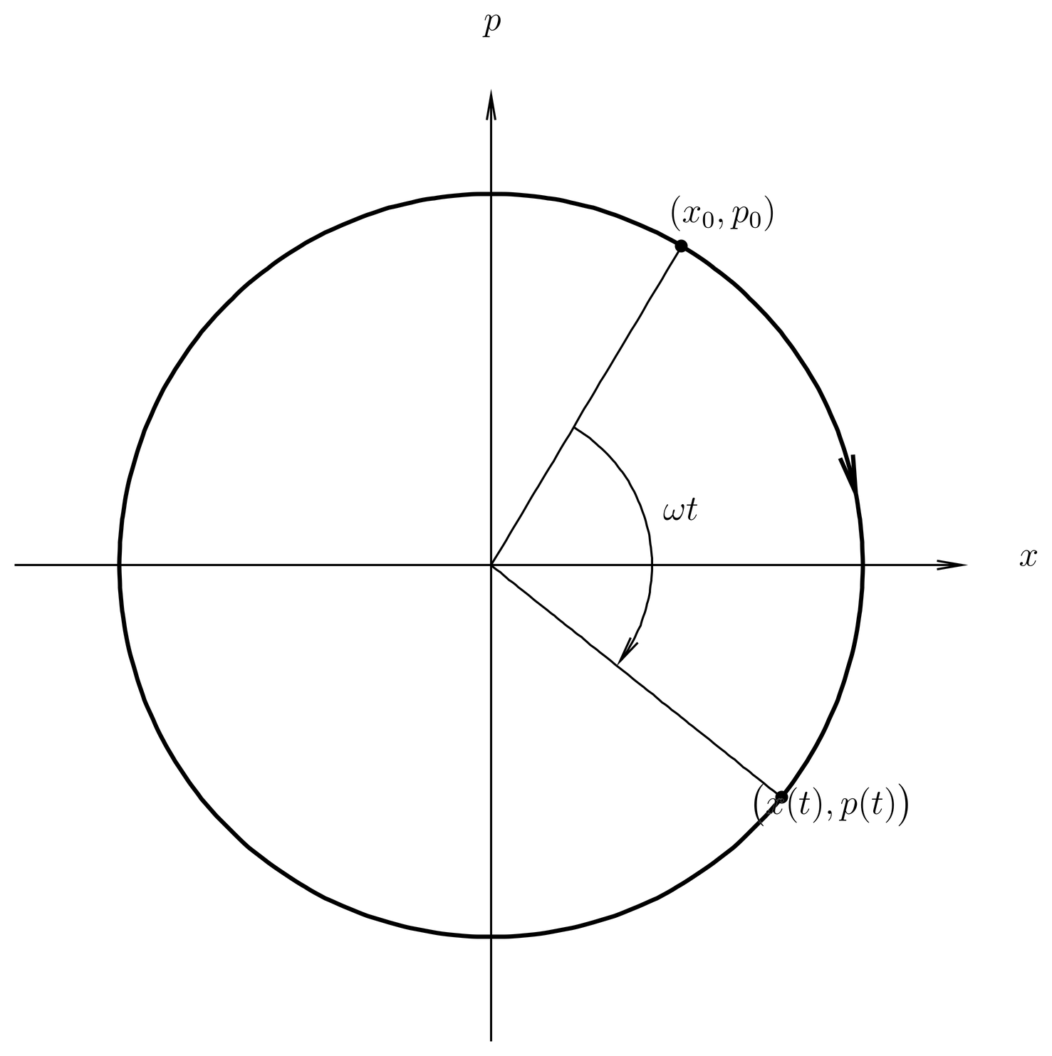
Figure 1:The classical motion in phase space is circular, in the clockwise direction.
The classical solution (52) is easily interpreted geometrically in phase space. The matrix shown is a rotation matrix in the - plane, in the clockwise direction for positive . Thus the phase point traces out a circle at unit frequency (or frequency if we restore ordinary units), as shown in Figure 1.
A certain set of complex variables is particularly nice for describing the classical motion. These are
where the overbar indicates complex conjugation. These are obviously classical versions of the annihilation and creation operators, defined in (17). These variables make the - phase plane into a complex plane, where and are proportional to the real and imaginary parts of . The classical Hamiltonian expressed in terms of these variables is , as shown in (16). The classical equations of motion in the variables are simply
with solution,
These are equivalent to (52). The phase factor causes the point in the complex plane to rotate in a clockwise direction as in Figure 1.
Similarly, the Heisenberg equations of motion for and can be written out,
and solved,
exactly as in the classical equations (55) and (56).
If is some state in the Heisenberg picture, we can take expectation values of both sides of (53) with respect to to obtain
Recall that expectation values are the same in the Heisenberg and Schr"odinger pictures, so this equation can be interpreted in the Schr"odinger picture if we like. We see that the expectation values follow the classical motion, as in (53) or Figure 1. See the discussion of the Ehrenfest relations in The Ehrenfest Relations.
Introduction to Coherent States
We shall discuss coherent states in the context of a one-dimensional harmonic oscillator, continuing with dimensionless units where . Coherent states in quantum optics are very similar from a mathematical standpoint, although the physical interpretation is quite different.
We define a coherent state as a wave function such that
Thus, the coherent state is a minimum uncertainty wave packet, since takes on its minimum value of . The expectation values of and can be anything, and serve as parameters of the coherent state. As shown in Minimum Uncertainty Wave Packets, a minimum uncertainty wave packet is always a Gaussian, and so also are the coherent state wave functions.
A common use of coherent states in the current literature is to explore the relationship between quantum and classical mechanics, and to obtain insight into the classical limit of a quantum system. In classical mechanics both and can be measured with infinite precision in principle, so the state of a classical system is defined by a point in phase space. In quantum mechanics, measurements of and display fluctuations about the average values and . The statistics of the fluctuations when measured across the ensemble are restricted by the uncertainty relations (54). But since a minimum uncertainty wave packet reduces these fluctuations to their minimum value, it is natural to regard a minimum uncertainty wave packet as the quantum object that comes as close as possible to a definite classical state.
The ground state of the harmonic oscillator (42) is an example of a coherent state, one for which . In a moment we will construct other coherent states with other values of and .
Minimum uncertainty wave packets satisfying (60) are not the only kind possible, for example, we could have
for which
A minimum uncertainty wave packet satisfying this condition is sometimes called a “squeezed state.” Actually, the wave function (61) is the ground state of a different harmonic oscillator than the one we have been discussing, one with different mass or frequency parameters. We cannot choose units so that for both oscillators, so the distinction between a coherent state (with equal position and momentum dispersions as in (60) and a squeezed state (with unequal dispersions) is only meaningful relative to a reference oscillator. In applications to quantum optics there is a natural reference oscillator, namely, the one describing a single mode of the electromagnetic field, whose excitations are identified with photons. In the case of mechanical problems, we must simply pick some reference oscillator. In the following we assume that the oscillator we started with, (11), with definite mass and frequency parameters, is the reference, and our definitions of coherent and squeezed states will be made relative to that reference.
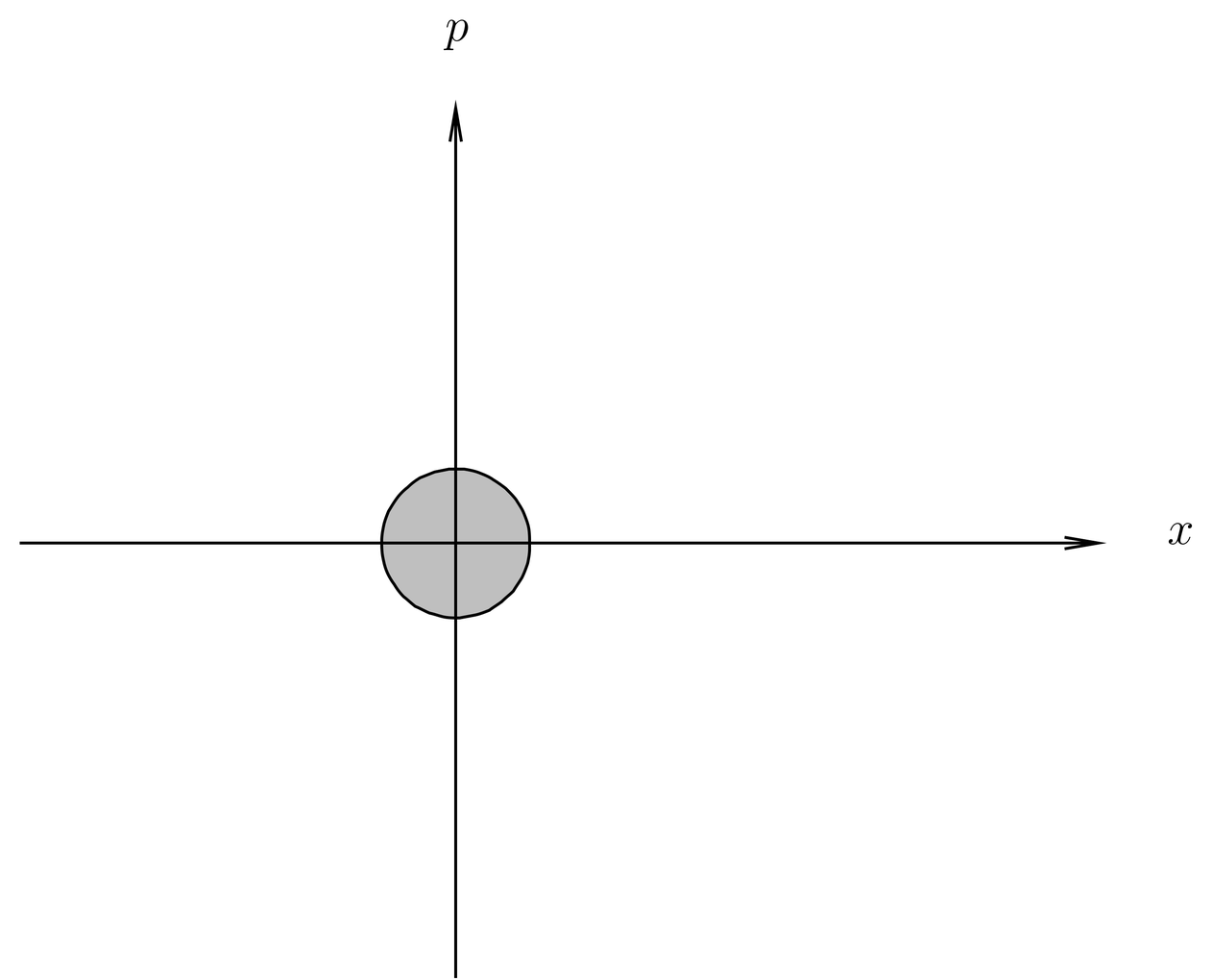
Figure 2:The ground state of the harmonic oscillator is seen as a circular blob in the classical phase space, centered on the origin.
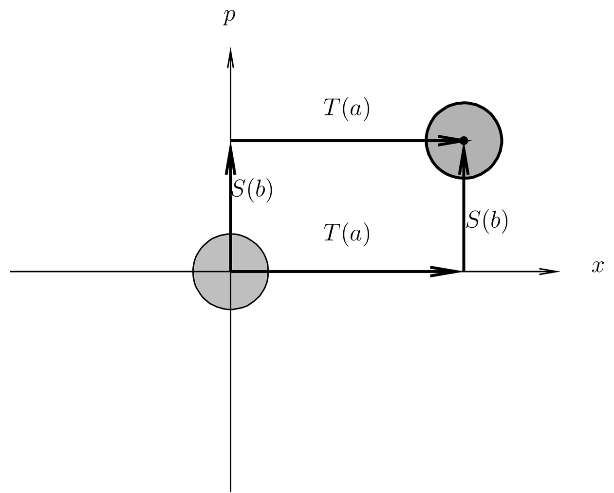
Figure 3:Operators and can be used to move the state to a new location in phase space.
It is useful to visualize the ground state of our harmonic oscillator as a circular blob in the classical phase space, as illustrated in Figure 2. This is not intended as a rigorous representation of the harmonic oscillator state, but merely as a picture that is useful for visualizing the fluctuations in the measurement process. We could make the picture more rigorous by introducing the Wigner function , discussed in Prob. Paragraph(d), but for simplicity we will not do that. We note, however, that the blob could be regarded as having an area of , the single Planck cell occupied by the quantum state.
To represent classical states with generally nonzero values of and , we would like to have minimum uncertainty wave packets with given values of and . These can be constructed from the ground state of the harmonic oscillator by means of translation operators in position and momentum. Translation operators in position were discussed in Translation Operators. In the present (dimensionless, one-dimensional) notation, they are defined by
where is the displacement. Their action on position and momentum space wave functions is given by
The operators have the following effect on expectation values. Let , , and let . Then and . We summarize these by writing,
The operator has no effect on the dispersions or . This fact is easily checked, but is plausible in any case since an ordinary probability distribution when displaced rigidly changes its mean but not its standard deviation.
Now we introduce the momentum displacement operators , defined by
which have the following effect on position and momentum space wave functions,
which may be compared to (64). The operators have the following effect on expectation values,
with no effect on the dispersions or . The cited properties of and are easily verified.
Since both and leave the dispersions and invariant, a minimum uncertainty wave packet is mapped into another minimum uncertainty wave packet by these operators, with new values of and . For example, the state can be thought of as a blob in phase space centered on , as illustrated in Figure 3.
Heisenberg Operators and Glauber’s Theorem
A minor problem, however, is that the operators and do not commute, something that is not surprising in view of the fact that they are exponentials of noncommuting operators. In detail, if we apply these operators in different orders to a wave function we get
or,
This means that the phase of the final state illustrated in Figure 3 depends on the order in which we apply and . In order to treat and on a more equal footing, we now introduce the Heisenberg operators, which carry out displacements in position and momentum simultaneously.
The Heisenberg operators are defined by
which may be compared to (63) and (66). The relation between the Heisenberg operators and the operators and is clarified by Glauber’s theorem, to which we now turn.
To prove this theorem, we introduce the $\lambda$-dependent operator $F(\lambda)$,

:::{math}
:label: eq-harmosc-71
F(\lambda) = e^{\lambda A} e^{\lambda B},
so that
But we know that
according to Prob. Paragraph(a). But since commutes with and , all terms in this series after the first two vanish. Therefore we have
If all symbols were numbers instead of operators, the solution, subject to initial conditions , would be
and we may take this as a guess for the solution of the operator problem. To verify that the guess is correct, we must check that the exponent in (76) commutes with its -derivative. This is straightforward to do. Finally, setting , we obtain the proof of the theorem. Glauber’s theorem has a fairly narrow scope, but it is useful in a number of applications.
We apply Glauber’s theorem to the product,
setting and , so that
The commutator is a -number, which commutes with everything, so the conditions of Glauber’s theorem are satisfied, and we have
or,
The Heisenberg operator just splits the phase between the two choices, and . It has the following effect on expectation values,
and leaves the dispersions and invariant.
We now define the coherent states by
The coherent state is parameterized by its expectation values and , and can be thought of as a blob centered on point in phase space as in Figure 3. The wave function of the coherent state is easily worked out; it is
The coherent states form a 2-parameter family of minimum uncertainty wave packets, that can be thought of as populating the entire phase plane. They have many interesting properties, for example, they form a complete set (but not orthonormal), so that an arbitrary wave function can be expressed as a linear combination of minimum uncertainty wave packets.
Time Evolution of Coherent States
Since a coherent state is the quantum state that is as close as we can come to a classical state, it is of interest to compare the time evolution of a coherent state in quantum mechanics to the corresponding classical time evolution. We know part of the answer already, for as shown in The Heisenberg Picture and Classical Equations of Motion, the expectation values of the time-evolved quantum state follow the classical motion. But does the initial coherent state remain a minimum uncertainty wave packet? And what about the other details of the quantum evolution?
To answer these questions, we will consider an initial state that is a coherent state, , where we make the replacements, , to represent an initial point in phase space. The coherent state itself can be thought of as a blob in phase space centered on , as in Figure 4.
We will determine the time evolution of this state under the harmonic oscillator Hamiltonian by expanding the initial state as a linear combination of harmonic oscillator eigenstates. The expansion can be achieved by using complicated identities involving Hermite polynomials and Gaussians, but an operator approach is much easier. We begin by casting the Heisenberg operator used to define the initial state into an alternative and useful form. This operator is
First, we adopt a complex notation for the points in phase space, exactly as in (54) but here referring to the initial point ,
and we use instead of to parameterize the coherent state as well as the Heisenberg operator:
Similarly, we use the creation and annihilation operators (see (17) instead of and . Then the exponent in the Heisenberg operator, a linear combination of and , becomes a linear combination of and :
We now apply Glauber’s theorem again, this time with and , so that . The commutator is a -number that commutes with everything, so the conditions of Glauber’s theorem are met and we have
or,
This is a form of the Heisenberg operator alternative to the form (84).
We now apply (89) to the ground state . Since all positive powers of annihilate , we have
As for the operator , we expand the exponential and use (40) to find
This is the desired expansion of the coherent state in terms of energy eigenstates. We see that the probability of finding the system in energy eigenstate is
This can be expressed in terms of the average energy of the coherent state , which we write as :
where the is the zero point energy and is the extra energy the coherent state acquires on being transported in phase space from to . Then the probability can be written
This makes it obvious that the probability is normalized,
In statistics, the distribution (94) is called a Poisson distribution. In quantum optics, it is the distribution of the number of photons in a coherent state. (It is customary to exclude the from the accounting of the energy of photons, as discussed in 41. The Quantized Electromagnetic Field.)
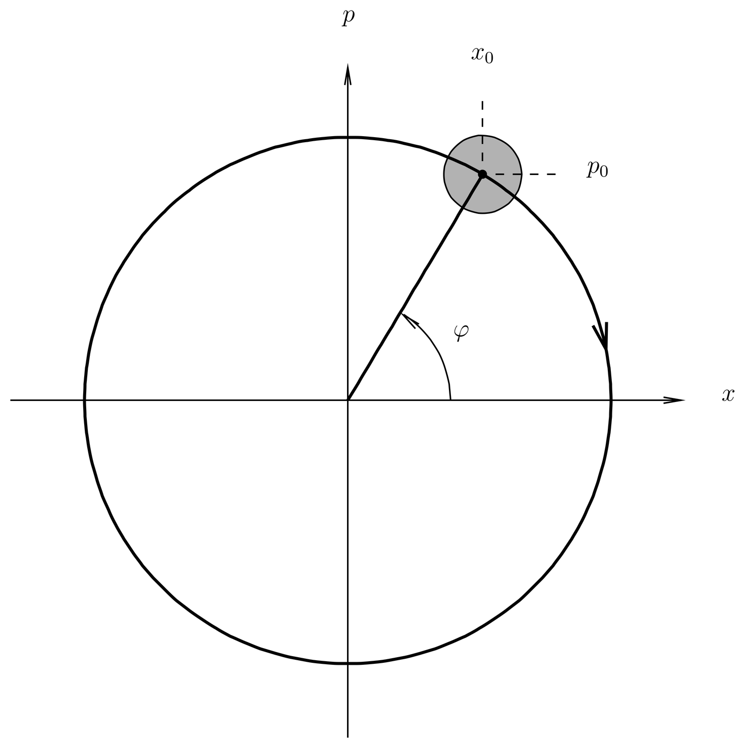
Figure 4:A coherent state can be used like the hands of a clock, to tell (approximately) the phase angle of the oscillator.
Obviously, the coherent state is not an energy eigenstate, except in the special case (the ground state of the harmonic oscillator). The expansion (91) illustrates an interesting version of the time-energy uncertainty principle, , since an energy eigenstate implies exact knowledge of , so that and . This means that in an energy eigenstate, we have no knowledge of the phase angle of the classical oscillator, illustrated in Figure 4, which could be used as a clock to tell the time. A correct semiclassical picture of an energy eigenstate is not a particle on an orbit or even a wave packet on an orbit as in Figure 4, but rather an object smeared out all along the classical orbit so as to give a uniform distribution in time. Recall the classical probability density in WKB theory, (51), which is uniform in time around the classical orbit. Since a coherent state such as illustrated in Figure 4 is localized in the phase angle it cannot be an energy eigenstate. Indeed, an alternative version of the time-energy uncertainty relation for harmonic oscillators is
where is the quantum number.
We can make a semiquantitative check of the relation (96) in the following way. From Figure 4, we can estimate by noting that since the radius in phase space is , and since , then . But from the Poisson distribution (92), we have , so (96) is verified. In the case of the quantized electromagnetic field, the number is identified with the number of photons, and the phase angle is identified with the phase of the electromagnetic wave in the usual sense in classical electromagnetic theory. Thus we see that in the quantized theory of the electromagnetic field, a state of well defined phase angle must be uncertain as to the number of photons it contains.
We can now easily find the time evolution of the coherent state. First we apply the time evolution operator to (91), using
to obtain
In this we see the appearance of , the solution of the classical equations of motion (see (56). and we note that . Thus we can write (98) as
where in the last step we have used (91) with replaced by . Therefore, to within the time-dependent phase , an initial coherent state remains a coherent state in the course of time in the harmonic oscillator, with the phase space parameters following a classical trajectory. The dispersions and are constant in time, retaining their values given by (60), and the wave packet remains a minimum uncertainty wave packet for all times.
A free particle Gaussian wave packet that is minimum uncertainty at spreads in time, with becoming arbitrarily large as , as shown in Prob. Paragraph. For these initial conditions, the wave packet also spreads as , that is, for negative times its width shrinks until it reaches the minimum uncertainty value at , after which it grows.
We have just shown, however, that in the case of the harmonic oscillator, an initial coherent state, a minimum uncertainty wave packet, remains minimum uncertainty with a constant value of as time advances. Another interesting case is when the initial state is a squeezed state. In this case it can be shown that under the time evolution generated by the harmonic oscillator, the width of the wave packet oscillates with twice the frequency of the oscillator itself, that is, the wave packet “breathes” periodically. This wave packet is minimum uncertainty, that is, it satisfies , at each integer multiple of a quarter period, while in between it satisfies . These facts can be shown either by operator methods or more direct methods based on solving the Schr"odinger equation.
In the case of Hamiltonians that are quadratic polynomials in and , such as the harmonic oscillator, not only are the Ehrenfest relations exact, but all the properties of the quantum time evolution bear an especially close relationship to the classical motion. For example, the spreading or breathing of wave packets can be understood in terms of ensembles of particles in the classical phase space.
Problems
Problem 1.
The eigenfunctions of the harmonic oscillator in configuration space are given by Eq.~(\eqr\cn.45). In this problem you may use dimensionless units, as described in Sec.~\secr\cn.3. Find the corresponding momentum space wave eigenfunctions, , which are defined by
Get the phases right.
Problem 2.
Consider the Hamiltonian for a particle of mass moving in the - plane,
An arbitrary potential that is quadratic in and and that has a minimum can be brought into this form by shifting the origin and rotating the axes, if necessary. The frequencies in the 1- and 2-directions are allowed to be different. You may know that the classical orbits in this case are Lissajous figures. The orbit is closed if the frequencies are commensurable.
The case in which is especially interesting. Two or higher dimensional oscillators with equal frequencies occur in many examples of molecular vibrations. In two dimensions this gives an example of two-dimensional central force motion,
since the potential is a function of the radius .
All central force problems in two dimensions have a symmetry, which is rotations in the plane. The generator of this symmetry is
It is the -component of angular momentum, and it is a constant of motion (see Constants of Motion) for any central force problem in two dimensions. But the two-dimensional, isotropic harmonic oscillator has further constants of motion, indicating a larger symmetry group than just rotations in the plane.
Let us choose units so that in (102). Then
Define creation and annihilation operators as in (17),
where we let Greek indices run over 1,2. These obey a generalization of the commutation relations (19),
which is just a statement that each oscillator has commutation relations like (19), and the variables of one oscillator commute with the variables of the other.
(a) Define number operators as in (21),
Then define further operators,
and
where are the Pauli matrices and .
Find the energy eigenvalues and degeneracies of the Hamiltonian (104), that is, find the spectrum of and the dimensions of the energy eigenspaces. Now let be an eigenvalue of . What are the allowed values of (that is, what is the spectrum of )?
(b) Show that if and are matrices of numbers, and if we define operators and by
then
Use this result to evaluate the commutators and . Explain why all three are constants of motion. Find a relationship between one of the and in (103).
(c) Show that
You may find it useful to use the identity,
which is the solution to Prob. Paragraph(d).
(d) Let and be the usual harmonic oscillator quantum numbers for oscillators 1 and 2 in (104), and let the energy eigenstates be . Show that is an eigenket of and . Express the eigenvalue of in terms of , and let the eigenvalue of be (not to be confused with the mass, which at this point we have set to unity). For a given value of , what values of are allowed?
You will see that this problem reproduces the beginnings of angular momentum theory. It can be extended to produce formulas for the Clebsch-Gordan coefficients, the rotation -matrices (see 13. Representations of the Angular Momentum Operators and Rotations), and many other things, with everything based ultimately on harmonic oscillator creation and annihilation operators.
Problem 3.
A problem on coherent states.
(a) Find convenient expressions for and , where is the Heisenberg operator (87) and and are the annihilation and creation operators. Hint: See Prob. Paragraph(a). Then show that the coherent state is an eigenstate of the annihilation operator with eigenvalue .
(b) The annihilation operator is not Hermitian, so its eigenvalues are not real in general, nor are its eigenstates orthonormal, that is, when . Nevertheless, they are complete in a certain sense. Prove that
This resolution of the identity shows that an arbitrary wave function can be expanded as a linear combination of coherent states, that is, Gaussian wave packets. However, the expansion is not unique, because the coherent states are actually overcomplete (they are not linearly independent). In fact, there are many vanishing linear combinations of coherent states (with nonzero coefficients). Nevertheless, the formula (114) looks neat. It can be used as the basis of a path integral.
(c) Use the Heisenberg picture to obtain expressions for and , where and are the usual annihilation and creation operators in the Schr"odinger picture, and is the time-evolution operator for the harmonic oscillator. Then use these to obtain a simple expression for
Finally, use that to obtain a simple expression for . This approach to finding the time evolution of a coherent state is easier than the one taken in the notes, which involved normal ordered Taylor series.
Problem 4.
Recoilless emission is an important part of the physics of the M"ossbauer effect. A simple one-dimensional model of the process is illustrated in Fig.~\figr\cn.5.
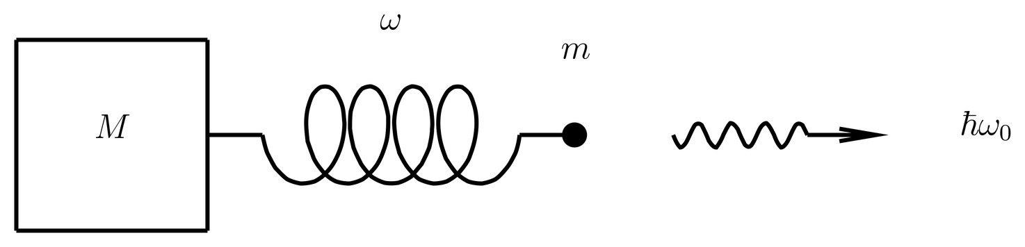
Figure 5:A simple one-dimensional model of an iron atom coupled to the modes of the crystal lattice. The emitted photon has energy , while the frequency of the spring is . The mass of the lattice is taken to . is the mass of the iron atom.
An iron atom of mass is attached by a spring to a large mass . The frequency of the harmonic oscillator is , while the frequency of the photon is . When the iron atom emits the photon, it suffers a recoil momentum whose magnitude is
Classically, we can say that the effect of the emission of the photon is to map the position and momentum of the iron atom according to
where .
If is the wave function of the iron atom before the photon is emitted, what is the wave function after the photon is emitted, that is, after the impulse indicated by (117) is delivered? Express your answer in terms of .
If the iron atom is initially in the ground state of the harmonic oscillator (), what is the probability that it will be found in state after the photon has been emitted? That is, what is the probability of the transition ? Express your answer as a function of and other parameters of the problem. Verify that the sum of probabilities is 1.
In particular, you will see that there is a non-zero probability for recoilless emission, .
You may find it convenient to carry out the calculation in units in which , where is the frequency of the harmonic oscillator (not to be confused with the frequency of the photon). If so, you should restore ordinary units in your final answer.