33. Elements of Atomic Structure in Multi-Electron Atoms
Introduction¶
In these notes we combine perturbation theory with the results of the Hartree-Fock calculation outlined in 32. The Hartree-Fock Method in Atoms{} to obtain a basic qualitative and semi-quantitative understanding of the low-lying energy levels and energy eigenfunctions in multi-electron atoms. We concentrate on the ground state configuration of low- atoms where -coupling is applicable. The presentation in these notes is based on the book Intermediate Quantum Mechanics by Bethe and Jackiw.
In these notes we continue with the custom of using the capital letters , and for the quantum numbers of the whole atom, while reserving lower case letters , , for those of a single electron.
Summary of the Results of Hartree-Fock Theory¶
In 32. The Hartree-Fock Method in Atoms{} we found a variational estimate to the ground state of the basic -electron atom Hamiltonian (1), reproduced here:
We denote the estimate for the ground state by ; it is a Slater determinant composed of single particle orbitals, , , as in (39). The individual orbitals are a product of a spatial part times a spin part, , where is the spatial wave function and is an assignment of spins (up or down) to each orbital. Once the Hartree-Fock equations have been solved, the orbitals specify the self-consistent direct and exchange potentials, and , according to (94) and (95), where the exchange “potential” is really the -space kernel of the operator that we call a potential.
We assume that these potentials have been averaged over spatial and spin rotations, as described in Averaging and the Electron Configuration, which causes and to be replaced by and , as in (104) and (105). The spatial parts of the orbitals are then solutions of the pseudo-Schr"odinger equation
where the effective single-particle Hamiltonian is
Here we denote the exchange potential, as an operator, by simply , recognizing that it is actually an integral transform.
Since the single-particle Hamiltonian is rotationally invariant, the single-particle orbitals are characterized by the standard set of central field quantum numbers for an electron, that is, . Also, the spatial part of the orbitals is given by
for some radial wave functions that are determined by solving the pseudo-Schr"odinger equation (2). Each orbital is associated with an energy , an eigenenergy of the Hamiltonian that only depends on the quantum numbers and , as usual for a central force problem.
The orbitals that go into the Slater determinant must be linearly independent, so the quantum numbers of the orbitals must be distinct. Since the orbitals are eigenstates of the single-particle Hamiltonian , they are, in fact, orthonormal. The Hamiltonian has an infinite number of eigenstates, so we must choose of them to form the Slater determinant and to compute the self-consistent potentials and while carrying out the iteration to solve the Hartree-Fock equations. When we obtain the Hartree-Fock estimate for the energy, the result will depend only on the quantum numbers , and not on the magnetic quantum numbers . Equivalently, the estimate for the energy will depend only on the number of occupied orbitals in each subshell. As explained in Averaging and the Electron Configuration, the list of occupation numbers is called the electron configuration.
Table 1:Electron configurations for some atoms. refers to the argon core, , while refers to the radon core, .
| Atom | Z | Config |
|---|---|---|
| H | 1 | |
| He | 2 | |
| Li | 3 | |
| Be | 4 | |
| B | 5 | |
| C | 6 | |
| N | 7 | |
| O | 8 | |
| F | 9 | |
| Ne | 10 | |
| Na | 11 | |
| Mg | 12 |
| Atom | Z | Config |
|---|---|---|
| K | 19 | |
| Ca | 20 | |
| Sc | 21 | |
| Ti | 22 | |
| V | 23 | |
| Cr | 24 | |
| Mn | 25 | |
| Fe | 26 | |
| Co | 27 | |
| Ni | 28 | |
| Cu | 29 | |
| Zn | 30 |
| Atom | Z | Config |
|---|---|---|
| Fr | 87 | |
| Ra | 88 | |
| Ac | 89 | |
| Th | 90 | |
| Pa | 91 | |
| U | 92 | |
| Np | 93 | |
| Pu | 94 | |
| Am | 95 | |
| Cm | 96 | |
| Bk | 97 | |
| Cf | 98 |
Different choices of electron configuration lead to different estimates of the ground state energy; we must choose the one that gives the smallest estimate. This gives the electron configuration for the ground state of the atom, as tabulated in references (for example, periodic tables of the elements). As we move from one atom to the next, the sequence of electron configurations reveals a filling sequence, that is, a sequence of subshells that are filled. See Table 1. For atoms of small , the sequence proceeds like this: , , , , etc. However, for heavier atoms there may be some competition between subshells, for example, in the transition elements the and subshells have nearly the same energy, so as we move from one element to the next, the next electron may go into the or subshell, whichever is energetically favorable, or it may go into the subshell while borrowing another electron from the subshell. This phenomenon was explained in terms of the exchange energy in The Hartree-Fock Energy Functional. Thus in the case of atoms of small the electron configuration for the ground state consists of a series of complete subshells plus a final subshell that may be incomplete, for example, carbon has the configuration , in which the subshell is incomplete (it has six orbitals but only two are filled). But heavier atoms such as the transition elements may have more than one incomplete subshell, for example, chromium has the configuration , in which the subshell with ten orbitals has only five filled, and the subshell with two orbitals has only one filled. We might mention that while in hydrogen the subshell has a higher energy than the , in heavier atoms the self-consistent potentials do not follow the rules of hydrogen.
Table 1 contains a partial table of electron configurations which shows these features of the subshell filling sequence. The table includes a list of low- atoms, a list of transition elements showing the competition between the and subshells, and a list of actinides, showing the competition between the , and subshells.
To summarize, for a given atom, Hartree-Fock theory, combined with averaging of the potentials, gives us an electron configuration; a set of self-consistent, rotationally invariant potentials and ; a set of eigenenergies ; and a set of single particle orbitals where . Actually, since the self-consistent potentials can be determined from the orbitals, it suffices just to give the orbitals; and since the orbitals are central force eigenfunctions as in (4), it suffices to just give the radial wave functions. For example, for carbon with configuration it suffices to give (in addition to the configuration) the radial wave functions , and and the eigenenergies , and . These radial functions and energies can only be found numerically.
The Central Field Approximation¶
The Slater determinant that emerges from Hartree-Fock theory is not only a variational estimate to the ground state wave function, it is also an exact eigenstate of the multi-particle Hamiltonian,
that is,
This is because each of the terms of the Slater determinant consists of the same orbitals, just permuted among the electrons, but brings out the total energy given by
which is invariant under permutations and is the same for all terms. Here in the last sum is the occupation number of subshell , that is, the number of electrons in that subshell. Note that although the ground eigenstate of is the Hartree-Fock estimate to the ground state eigenfunction of the atom, is not the Hartree-Fock estimate to the energy, since it double counts the direct and exchange potential energies among the electrons. See (100), which shows that is too high. We will show how to correct this energy in a moment.
The Hamiltonian represents what is called the central field approximation to the atom. It is a cruder model than the basic -electron atom Hamiltonian (1). It has more symmetry than that Hamiltonian, which is invariant under spatial rotations of the entire -electron system, generated by , but not under spatial rotations of the individual electrons, generated by the individual angular momenta . The central field Hamiltonian , however, is invariant under the rotations of individual electrons, that is, it commutes with each individually. It is a general rule in applications of quantum mechanics that the more idealized the model, the more symmetry there is and thus a higher degree of degeneracy. We will examine the degeneracy of in more detail below.
Coupling Schemes¶
We can make the central field Hamiltonian the basis of a perturbation expansion by writing , where
Here is the central field Hamiltonian (5) and is written so that is the basic -electron atom Hamiltonian (1). That is, we have added and subtracted the direct and exchange potentials inside to make .
The term in (9) consists of the exact interelectron Coulomb interactions, that is, the term , minus the rotational average of the direct minus exchange potentials, summed over electrons. This is sometimes called the “residual Coulomb potential.” If the rotational averaging provides a good approximation to the exact interelectron Coulomb interactions, then the term should be much smaller than the exact interelectron interactions. The exact interelectron Coulomb interactions are too big to treat by perturbation theory (apart from the case of helium, where the results are not very satisfactory from a numerical standpoint), but with the rotational average subtracted off, the result, the term above, is small enough for a successful perturbation treatment. That is, we have . We shall outline this perturbation treatment below.
But if is now a small term, the question arises, how does it compare to other small terms we have neglected so far, such as the fine structure terms? To take these into account as well, we shall contemplate another term in the Hamiltonian,
which is the sum of the spin-orbit interactions for each electron. The quantity is a function of the radius of the electron (see (13) whose details will not concern us. The spin-orbit term is only one of several fine structure terms, most of which we are omitting for simplicity, and even the spin-orbit term is treated somewhat schematically. Our goal will be to give a qualitative understanding of the effects of the fine structure terms without going into detail.
But to return to the question posed, what is the quantitative relation between and ? It turns out that the answer depends on . In low atoms near the beginning of the periodic table, we have . For such atoms, it makes sense to first treat as a perturbation on , find the eigenstates of , then to treat as a second perturbation on top of . This scheme involves classifying the eigenstates of by their good quantum numbers, including and , as discussed in Good Quantum Numbers of the Basic -electron Atom Hamiltonian below. This scheme is called - or Russell-Saunders coupling. For high atoms, however, near the end of the periodic table, it turns out that . In this case it makes sense to first treat as a perturbation on top of , then to treat as a perturbation on top of . This scheme is called -coupling, on account of the quantum numbers that arise in it. In these notes we consider only -coupling.
The Unperturbed System in -Coupling¶
Let us therefore consider as a perturbation on top of . As usual in perturbation theory, we must first understand the unperturbed system, its eigenstates and eigenvalues, and in particular its degeneracies, since those affect how the perturbation calculation is carried out. The ground state energy of is , shown in (7), and the Slater determinant composed of central field orbitals is a ground state eigenfunction of . Each subshell contains orbitals, each of which has the same energy , but not all the orbitals are necessarily occupied by electrons. In complete subshells, in which all the orbitals are occupied, there is only one way to assign orbitals to the electrons. But if there are any incomplete subshells, then there is more than one way to assign central field orbitals without changing the energy , since the energy does not depend on the assignment of magnetic quantum numbers to the orbitals. Thus, if there are any incomplete subshells, the ground state of is degenerate, and the degenerate eigenfunctions are the Slater determinants specified by the choices of magnetic quantum numbers for the orbitals in incomplete subshells.
To distinguish the various Slater determinants with different magnetic quantum numbers, we will replace the notation with , where “-set” refers to the magnetic quantum numbers in incomplete subshells only. We do not need to specify the magnetic quantum numbers in complete subshells, since there is only one possible assignment for those. Here the electron configuration is understood, which specifies which subshells are incomplete and how many electrons they contain. In the equation,
a version of (6), the energy depends on the configuration but not on the -set, and the order of the degeneracy is the number of possible -sets.
Notice that in assigning orbitals to electrons the order of the assignment does not matter, since all electrons are permuted among all orbitals by the Slater determinant. All that matters is which orbitals are assigned, that is, the list of assigned orbitals. More precisely, if we change the order in which the orbitals are assigned to the electrons, the Slater determinant will change sign if the rearrangement of the orbitals amounts to an odd permutation. Apart from this sign, the order does not matter, and even the sign is pinned down if we put the orbitals in a standard order when assigning them. Therefore the number of distinct assignments of electrons to orbitals in a subshell containing slots is the binomial coefficient , which is the number of distinct unordered subsets of elements taken from a set of elements. This is the number of distinct -sets possible for the given subshell. As explained above, for low atoms the electron configuration has only one incomplete subshell, so the degeneracy of the ground state is a single binomial coefficient for that subshell. For heavier atoms there may be more than one incomplete subshell, in which case the degeneracy is the product of the binomial coefficients, one for each incomplete subshell.
Enumerating -sets¶
Consider, for example, B (boron), with electron configuration . There is one electron in the one incomplete () subshell. Since this subshell contains slots (for ), there are six possible -sets, and the ground state energy is six-fold degenerate. The degeneracy is given by the binomial coefficient,
See Table 2.
Table 2:Allowed -sets for boron, with configuration .
| 1 | 1 | |
| 2 | 1 | |
| 3 | 0 | |
| 4 | 0 | |
| 5 | -1 | |
| 6 | -1 |
Now consider carbon, with configuration , whose -sets are listed in Table 3. There are now two electrons in the incomplete subshell, so the degeneracy is
Since there are two electrons, there are now two and two values in an -set. The table lists all combinations of pairs in descending order, that is, such that . For example, the table contains but not , which is just an exchange of quantum numbers that does not represent a distinct state. When the two values are equal, for example, in row~1 of the table where , then only one set of values is given, namely, , because if then the state vanishes, and because is the same state as . But if the values are distinct, as for example in rows~2--5 of table where , then all combinations of values are given, because they all represent distinct states. Proceeding in this way the table lists all possible -sets, confirming that there are 15 total.
Table 4:Allowed -sets for nitrogen, with configuration .
| 1 | 1 | 1 | |||
| 2 | 1 | 1 | |||
| 3 | 1 | 1 | |||
| 4 | 1 | 1 | |||
| 5 | 1 | 0 | |||
| 6 | 1 | 0 | |||
| 7 | 1 | 0 | |||
| 8 | 1 | 0 | |||
| 9 | 1 | -1 | |||
| 10 | 1 | -1 |
| 11 | 1 | 0 | |||
| 12 | 1 | 0 | |||
| 13 | 1 | 0 | |||
| 14 | 1 | 0 | |||
| 15 | 1 | -1 | |||
| 16 | 1 | -1 | |||
| 17 | 0 | 0 | |||
| 18 | 0 | 0 | |||
| 19 | 0 | -1 | |||
| 20 | 0 | -1 |
As a final example, consider nitrogen, with configuration . The number of -sets is
These are listed in Table 4. The triplets are listed in descending order, that is, , but triplets with the same values, that is, , are omitted, since for those it is impossible to assign electron spin quantum numbers without creating a duplicate and hence a zero state. In cases where two ’s are equal and one different, for example, rows~1--2 with , the identical values are matched with and , and the odd is matched with , giving a total of two states. In cases where all three ’s are distinct, for example, rows~7--14 of the table for which , all possible values are assigned, giving distinct states. The number of distinct -sets in the table is 20, agreeing with the binomial coefficient (14).
Good Quantum Numbers of the Basic -electron Atom Hamiltonian¶
We see that if the electron configuration contains any incomplete subshells then the ground state of is degenerate. This means that we can expect the ground state of to split when the perturbation is turned on, and that in principle we will have to diagonalize a matrix to find the energy shifts. As usual in perturbation theory, it helps to employ a basis in the perturbation calculation that is an eigenbasis of a set of commuting operators, in which as many as possible of the operators commute with the perturbation. See Choosing a Good Basis in Degenerate Perturbation Theory. In the present case, the operators that commute with are the same that commute with , that is, the operators in question commute with the basic -electron Hamiltonian (1).
These operators were discussed in The Basic -electron Hamiltonian, and include , and . If we ask for a list of operators that commute with and with each other, then a suitable choice is , , , and . Thus the eigenstates of can rigorously be characterized by their quantum numbers (using both for the parity operator and its eigenvalue). The Slater determinant , however, is an eigenstate only of , and , and not, in general, of and .
To see this consider first
the -component of orbital angular momentum, summed over all the electrons. When this is applied to a single term in a Slater determinant , each operator brings out the value , the ~value of the orbital assigned to electron in the given term. Thus brings out the sum of these values, . There are terms in the Slater determinant, but these consist of permuting orbitals among electrons, and this sum is invariant under such permutations. Thus the sum is the same for all the terms of the Slater determinant, and we have
Similarly, we have
As for parity, the operator maps all position vectors into , and so brings out a factor from the orbital with angular momentum quantum number . The product of these factors is invariant under permutations and therefore the same for all the terms of the Slater determinant, and we have
The parity eigenvalue depends only on the electron configuration, which specifies the quantum numbers for all the electrons. In the following discussion we will be concentrating on the fixed ground state configuration of an atom, so the parity quantum number will be fixed and will not play a large role in the subsequent considerations.
In summary, the Slater determinant composed of central field orbitals is an eigenstate of , and with quantum numbers
Actually, the sums and products in these eigenvalues can be taken over incomplete subshells only, since the sums and are 0 when taken over complete subshells, and the product is 1 when taken over complete subshells. Thus, the eigenvalues of and depend only on the -set. As for the parity , it is independent of the -set and depends only on the configuration.
A similar argument does not work, however, for the operators and . The individual terms of a given Slater determinant are not in general eigenstates of these operators, and neither is the sum. The Slater determinants , for the -sets allowed by the configuration, span the ground eigenspace of , but they diagonalize only the symmetry operators , and , not and .
A Symmetry Adapted Basis¶
Let us denote the ground eigenspace of by . This space is spanned by the Slater determinants , where the -sets run over all allowed by the incomplete subshells (for example, 15 in the case of carbon). Thus in first order perturbation theory we need in principle to diagonalize the matrix to find the energy shifts, which give us the energy eigenvalues of that grow out of as is switched on.
This matrix may be large (for example, it is in the case of carbon), so it will help to choose a good basis to simplify the diagonalization. The best basis is an eigenbasis of a set of commuting, good quantum numbers, such as , as discussed in Good Quantum Numbers of the Basic -electron Atom Hamiltonian. We omit from the list since it is constant on (all basis states have the same parity). The set of Slater determinants is not such a basis, since it is not an eigenbasis of or , in general.
The operators commute with and so can be restricted to (see Simultaneous Eigenbases of Commuting Observables). Also, since they commute with each other, they possess simultaneous eigenspaces inside . These simultaneous eigenspaces are characterized by the quantum numbers of the operators . If any of these eigenspaces are multidimensional, that is, if there is any degeneracy inside remaining after the quantum numbers are specified, then we can introduce an index to label an arbitrarily chosen orthonormal basis inside the eigenspaces. In this way we conclude that there is an orthonormal basis inside that we can label by . Furthermore, we can show that if , and are held fixed, then the basis vectors with different values of and are related by the raising and lowering operators, and . This is a way of saying that breaks up into irreducible subspaces under both purely orbital and purely spin rotations, which in turn is a consequence of the fact that is invariant under both orbital and spin rotations.
Actually, as it turns out, for small the simultaneous eigenspaces of inside are nondegenerate, so the index is not needed. The first element for which such a degeneracy appears is vanadium, with . For simplicity in the following we will suppress the index , since the examples we will deal with have (but see Prob.~\prbratomstruc-1).
So to find a good basis for perturbation theory, we must find the basis vectors inside as linear combinations of the Slater determinants . We write these linear combinations schematically as
Once we have found the coefficients, then we can compute the matrix elements of inside with respect to the new basis,
Since commutes with all of the operators , it is diagonal in the basis and the energy shifts are the diagonal elements (21). (The off-diagonal elements vanish, and there is no need for primes on one side or the other in (21).) Moreover, since is invariant under both spatial and spin rotations, the energy shifts do not depend on the quantum numbers or . Thus, after the perturbation is turned on, the energies depend on and , and are -fold degenerate. In general, the unperturbed energy level will split into more than one energy level, each characterized by a value of and .
The values of and that occur for a given atom are called multiplets. These are the energy levels of low- atoms that are seen experimentally, at a resolution at which fine structure can be ignored. Understanding the multiplets, such as which ones occur and in what order, constitutes a basic understanding of the structure of multielectron atoms.
Determining the coefficients in the expansion (20) is somewhat like the problem of finding Clebsch-Gordan coefficients, but it is more complicated because there are two distinct kinds of angular momenta, orbital and spin, because the number of individual angular moments (the and for the electrons in the incomplete subshells) that must be added is in general more than two, and because of the requirements of antisymmetry. Still, it is not that hard (see Prob.~\prbratomstruc-2). For the time being, however, we shall concentrate on a simpler problem, which is to determine which multiplets (which values of and ) occur in . This is necessary in any case before we can compute the coefficients in (20).
Determining the Multiplets¶
The spectroscopic notation for a multiplet with given and is , where is replaced by one of the code letters, , , , , etc., for . We will now determined the multiplets inside the ground state eigenspace of for several different atoms.
For any atom with complete subshells, for example, beryllium with configuration or neon with configuration , there is only one multiplet, (that is, and ), which is pronounced, “singlet-.” For such atoms, there is only one way to assign orbitals to electrons, and therefore only a single Slater determinant, which spans the one-dimensional eigenspace . Now since is invariant under both spatial and spin rotations, it must break up into irreducible subspaces under both kinds of rotations. But a one-dimensional space can only hold the value 0 of angular momentum, since all higher values have multi-dimensional irreducible subspaces. Therefore only the values and are allowed.
In atoms with incomplete subshells, the allowed multiplets are determined by the incomplete subshells only. This is because the other (complete) subshells have and , which do not contribute to the total and of the atom.
In the case of boron there is one electron in the incomplete shell , and the -sets are given in Table 2. The total orbital and spin angular momentum of the atom are the same as the orbital and spin of this one electron, that is, and . Thus there is one multiplet, (pronounced “doublet-”). It has a degeneracy , the same as the binomial coefficient (12).
Table 5:Multiplets in the ground configuration of carbon.
| multiplet | degen | ||
|---|---|---|---|
| 0 | 0 | ||
| 1 | 1 | ||
| 2 | 0 | ||
| total | 15 |
In the case of carbon there are two electrons. We can determine the allowed multiplets by a special method that only works for two equivalent electrons. Here the word “equivalent” means, belonging to the same subshell. Both electrons have . When we combine two angular momenta , we obtain , that is, , 1 or 2. Of these, is symmetric under exchange of the electrons, is antisymmetric, and is symmetric. In general, when we combine two angular momenta, the maximum value of total angular momentum is symmetric under exchange, and the exchange symmetry alternates as we decrease that value down to 0. See Prob. Paragraph. Similarly, when we combine the spins of the two electrons, we get , that is or , of which is symmetric under exchange of electrons and is antisymmetric. Now since the overall wave function must be antisymmetric, we can have a state that is symmetric under orbital exchange and antisymmetric under spin exchange, or vice versa. Thus the possibilities are , , or ; and , or ; and and , or . These multiplets are pronounced, “singlet-,” “triplet-,” and “singlet-.” These possibilities are enumerated in Table 5 along with the degeneracies, that is, the dimensionalities of the subspaces of a given multiplet. These dimensionalities add up to 15, as they must.
We now present a tabular way of getting the multiplets for carbon which can be generalized to more than two equivalent electrons. Table 6, which is an expanded version of Table 3, shows the work. The logic is similar to that employed in the determining the allowed values of and when coupling angular momenta (see Allowed Values of and ).
Table 6:A tabular way of getting the multiplets in carbon.
| multiplet | degen | |||||||||
|---|---|---|---|---|---|---|---|---|---|---|
| 1 | 1 | 1 | 1/2 | -1/2 | 2 | 0 | 2 | 0 | ||
| 2 | 1 | 0 | 1/2 | 1/2 | 1 | 1 | 1 | 1 | ||
| 3 | 1 | 0 | 1/2 | -1/2 | 1 | 0 | ||||
| 4 | 1 | 0 | -1/2 | 1/2 | 1 | 0 | ||||
| 5 | 1 | 0 | -1/2 | -1/2 | 1 | -1 | ||||
| 6 | 1 | -1 | 1/2 | 1/2 | 0 | 1 | ||||
| 7 | 1 | -1 | 1/2 | -1/2 | 0 | 0 | ||||
| 8 | 1 | -1 | -1/2 | 1/2 | 0 | 0 | ||||
| 9 | 1 | -1 | -1/2 | -1/2 | 0 | -1 | ||||
| 10 | 1 | 0 | 1/2 | -1/2 | 0 | 0 | 0 | 0 | ||
| 11 | 0 | -1 | 1/2 | 1/2 | -1 | 1 | ||||
| 12 | 0 | -1 | 1/2 | -1/2 | -1 | 0 | ||||
| 13 | 0 | -1 | -1/2 | 1/2 | -1 | 0 | ||||
| 14 | 0 | -1 | -1/2 | -1/2 | -1 | -1 | ||||
| 15 | -1 | -1 | 1/2 | -1/2 | -2 | 0 | ||||
| total | 15 |
The 15 -sets for carbon are listed and numbered in the first five columns of the table, after which follow two columns with the and values. The method begins with row 1, an -set with and . This is the highest value in the table, and is the highest (actually, the only) value that occurs with . Therefore this -set is a nondegenerate simultaneous eigenstate of and with eigenvalues 2 and 0, respectively. Now since and both commute with and , this state must be an eigenstate of both and , according to Theorem Theorem. But what are the quantum numbers of and , that is, what are and ? First, cannot be less than 2 because that would violate the rule . Nor can be greater than 2, because if it were, we could apply a raising operator to this state and obtain a state with . But there is no state with . Therefore we must have . A similar logic shows that must be 0 for this state. This means that -set number 1 is the doubly stretched state of a multiplet with and , that is, the multiplet , as shown in the table. The multiplet is marked with the symbol \S.
This multiplet has states in it, which can be obtained by applying the lowering operators and to the doubly stretched state. Actually, in this case, we need only apply , since . Applying once gives a state with and . Now there are two -sets with these values of and , numbers 3 and 4, and number 3 is marked with the symbol \S, meaning . This does not mean that if we apply to the -set number 1 we get -set number 3. It means that -sets 3 and 4 span a 2-dimensional space, and if we apply to -set number 1 we get a vector in this space, that is, a linear combination of -sets numbers 3 and 4. Applying again we get a state with , , which must lie in the 2-dimensional space spanned by -sets numbers 7 and 8. The first of these is marked with \S. Similarly we mark -set 12 with \S, indicating one vector in the 2-dimensional space spanned by -sets 12 and 13, with and , and finally we mark -set 15 with \S, which spans the 1-dimensional space with and .
Next we look for the -set in the table that is not marked with \S{} that has the highest and values. We find it in -set number 2, which has and . This must be the doubly stretched state of a multiplet with and , that is, a multiplet. We mark this -set and all 8 others that can be obtained from it by applying and with the symbol \dag. Finally, we look for -sets that are not marked either with \S{} or \dag{} and we find -set number 10, the doubly stretched state of a multiplet with and , that is, the multiplet. It has only one state, which is marked with \ddag. In this way, we find the same multiplets for carbon as were given in Table 5.
Table 7:for obtaining the multiplets in nitrogen.
| Multiplet | degen | |||||||||||
|---|---|---|---|---|---|---|---|---|---|---|---|---|
| 1 | 1 | 1 | 0 | 1/2 | -1/2 | 1/2 | 2 | 1/2 | 2 | 1/2 | (§) | |
| 2 | 1 | 1 | -1 | 1/2 | -1/2 | 1/2 | 1 | 1/2 | ||||
| 3 | 1 | 0 | 0 | 1/2 | 1/2 | -1/2 | 1 | 1/2 | 1 | 1/2 | (†) | |
| 4 | 1 | 0 | -1 | 1/2 | 1/2 | 1/2 | 0 | 3/2 | 0 | 3/2 | (‡) | |
| 5 | 1 | 0 | -1 | 1/2 | 1/2 | -1/2 | 0 | 1/2 | ||||
| 6 | 1 | 0 | -1 | 1/2 | -1/2 | 1/2 | 0 | 1/2 | ||||
| 7 | 1 | 0 | -1 | -1/2 | 1/2 | 1/2 | 0 | 1/2 | ||||
| total | 20 |
The tabular method can be applied to nitrogen, with 3 equivalent electrons. A simplification is to notice that if all we want are the multiplets, it suffices to list only the -sets with and , since the multiplets are identified by their doubly stretched states. In the case of nitrogen, this only requires us to list 7 -sets out of 20. These are shown in Table 7. The multiplets are , and (pronounced, “quartet-”), and the degeneracies add up to 20, as they must.
After nitrogen we come to oxygen with configuration , which has four occupied orbitals in the subshell and two unoccupied ones, or, as we say, two “holes.” Some experience with constructing tables as above shows that holes lead to the same multiplets as electrons. Therefore the multiplets for oxygen are the same as for carbon, that is, , and . Similarly, fluorine, one hole in the subshell, has the same multiplet as boron, namely, , and neon, with all subshells filled, has the one multiplet .
Hund’s Rules and Fine Structure¶
Figure 1 shows the low-lying energy levels of carbon. The levels shown are experimental, but at the resolution of the diagram they are identical to the multiplets of the basic -electron Hamiltonian (1). That Hamiltonian omits a number of small effects such as fine structure, but those are too small to be seen at the scale of the diagram. At higher resolution, however, many of the levels of the diagram will be seen to be split. The levels are labeled by the configuration they belong to, with even parity configurations on the left and odd ones on the right. The three multiplets we found in Tables~Table 5 and Table 6 are the three lowest levels, all of even parity, labeled as belonging to the ground state configuration . One can see that this configuration is reasonably well separated from other (excited state) configurations.
The theory we have presented so far tells us the multiplets in the ground state configuration, but not their energies or even the ordering of the energies. These of course can be obtained by explicitly evaluating the matrix elements (21). It turns out that when there is only one multiplet, for example, in the case of complete subshells, then the energy estimate coming from first order perturbation theory agrees with the Hartree-Fock estimate (see Prob. Paragraph), while if there is more than one multiplet, then the one with minimum energy is less than the Hartree-Fock estimate but still an upper bound to the true ground state of the Hamiltonian (1). In Figure 1 we see that the ground state multiplet for carbon is .
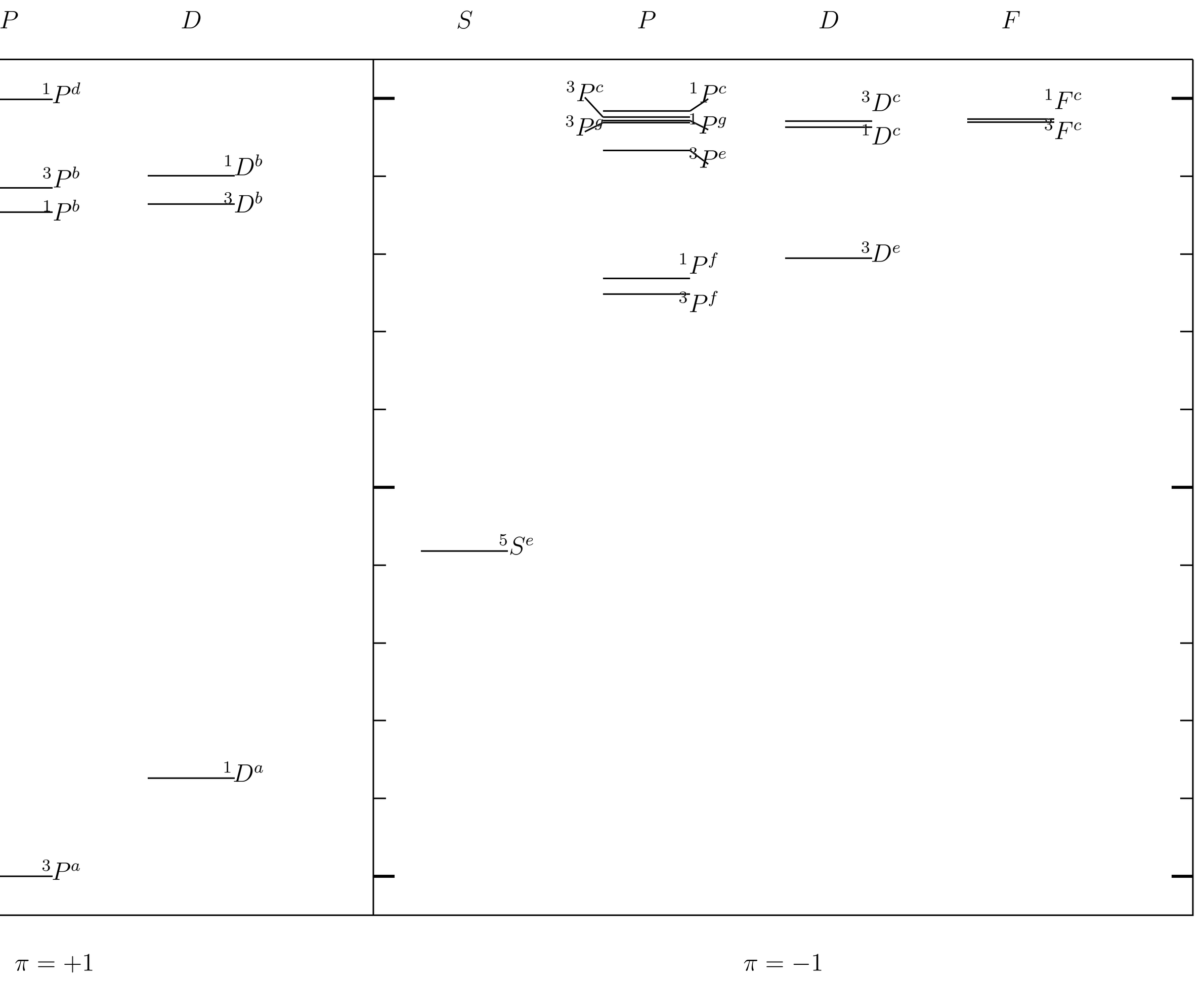
Figure 1:Atomic energy levels of carbon. Energies are measured in eV from the ground state, and all levels less than are shown. Levels of even parity () are on the left, those of odd parity () on the right. The superscripts , , etc, refer to the electron configuration, with , , , , , , . All configurations are understood to be attached to a helium core, . Source: NIST database.
A set of semi-empirical rules, called Hund’s rules, tell which multiplet in the ground state configuration has the least energy (this is the ground state multiplet). Hund’s rule number~1 says that the ground state multiplet has the highest value of among all the multiplets in the ground state configuration. For example, in the case of carbon, the multiplet has the highest , and we see that it is the ground state. Higher leads to lower energy because it implies that the individual spins are aligned, which in turn means that the spin part of wave function is symmetric, which implies that the spatial part of the wave function is antisymmetric. This keeps the electrons further apart, lowering their Coulomb energy. This is the same reason that the triplet states are lower in energy than the singlet states in helium, as explained in Perturbation Analysis of the Excited States. In case there is more than one multiplet with the highest value of , Hund’s rule number~2 says that of these, the one with the highest has the lowest energy.
When we apply the fine-structure perturbation (see (10) on top of , we see that in general we will have degenerate perturbation theory, in which we must contemplate diagonalizing the matrix
Here it is understood that we are working in the ground state configuration, and that and specify a unique multiplet (so that the index is not needed). The indices and are the same on both sides of the matrix element, because they specify the multiplet, that is, the eigenspace of the Hamiltonian , while the and indices are allowed to be different because they specify the basis inside that unperturbed eigenspace. The matrix is not diagonal in or because and , which generate respectively rotations of all orbital and all spin degrees of freedom, do not commute with .
This is potentially a large matrix, for example, it is in the case of the ground state multiplet of carbon. But the strategy for diagonalizing it is (by this time) obvious: we must switch from the uncoupled basis to the coupled basis , in which . The total angular momentum generates rotations of all degrees of freedom of the system, so it commutes with . Therefore we define
where the last matrix element is a Clebsch-Gordan coefficient, and now the energy shifts are just the diagonal matrix elements with respect to the coupled basis,
and they are independent of as indicated. The new energy levels are -fold degenerate.
For example, in the case of the ground state multiplet of carbon, in which and , we have , 1 or 2. We see that the 9-dimensional multiplet breaks up into three subspaces when fine structure is turned on, of dimensionality 1, 3 and 5. These are the energy levels of , called terms. Terms are denoted in spectroscopic notation. For example, in the case of the ground state multiplet of carbon, the terms are , and .
The theory presented does not allow us to say which term in the ground state multiplet has the lowest energy, but Hund’s rule number ~3 comes to the rescue. This rule says that in configurations in which the incomplete subshell is less than half filled, the term with the lowest energy is the one with the lowest . These are called regular multiplets. But if the incomplete subshell is more than half filled, then the term with the least energy is the one with the highest . These are called inverted multiplets. For example, in the case of carbon, for which the subshell is less than half filled, the ground state term is . But in oxygen, which as the same multiplets as carbon (because holes behave the same as electrons, insofar as determining multiplets is concerned), the ground state term is . These ground state terms give the exact quantum numbers of the true ground state of .
In the case of multiplets in which the incomplete subshell is exactly half filled, such as nitrogen, first order perturbation theory for the terms gives a vanishing result, and one must go on to second order theory. We omit the details.
Problems¶
Problem 1.
Work out the multiplets which result from 3 equivalent electrons. (``Equivalent’’ means that they all belong to the same subshell.) Check to make sure your answer adds up to the correct number of levels, based on the degeneracy expected in the central field approximation. You will see the necessity of the index in , since some multiplets appear more than once. In the case of vanadium, use Hund’s rules to determine the ground state multiplet. When spin-orbit coupling is turned on, the multiplets split, and the resulting levels are denoted . Which of these represents the ground state of vanadium?
Problem 2.
Write out the wave functions explicitly for an configuration (e.g., nitrogen), that is, as linear combinations of Slater determinants that you may identify by their -sets (the set of magnetic quantum numbers for electrons in incomplete subshells). To help the grader, use the same ordering of magnetic quantum numbers as shown in Table~\tblr\cn.4, for example, denote Slater determinant number~5 in that table by .
Table 4 effectively gives a standard ordering for the orbitals in the Slater determinant, one in which and in which the values corresponding to a run of equal values are in descending order. Since there can be a maximum of two values in a row that are equal, that means for the corresponding values in that case. This rule is followed in the table.
Problem 3.
A problem on -coupling. The Hamiltonian (in atomic units) for a neutral atom () can be written , where the three terms are given by Eqs.~(\eqr\cn.8a), (\eqr\cn.8b) and (\eqr\cn.9).
The energy eigenvalues of are determined by the electron configuration. We will be interested in lead (Pb, ), with two electrons outside closed subshells, and bismuth (Bi, ), with three electrons outside closed subshells. For such heavy atoms, is larger than , so we first solve the Hamiltonian , then successively add the terms and , and see what happens to the energy levels and eigenstates.
We can assume that is solved for the ground state configuration, and that it gives a known energy . This would involve Hartree-Fock theory, and would give us the central potential . Next we add and write
where
We write the single particle eigenstates and eigenvalues as
where stands for the single particle quantum numbers , and where is independent of , . The states form an orthonormal basis in the Hilbert space for a single electron. The eigenstates of are Slater determinants formed out of orbitals , and the corresponding energies are
The terms in the last, incomplete subshell, the with , have two possible values, and . So the contribution from the last subshell depends on the number of electrons with and the number with .
For example, in Pb with the configuration, the two electrons can give three possible pairs of values, , , or . Therefore the single level of breaks up into three levels , labeled by , when we turn on . As we know from spin-orbit theory (25. Fine Structure in Hydrogen and Alkali Atoms), the energy is an increasing function of , so the are sequenced as indicated in Figure 2.
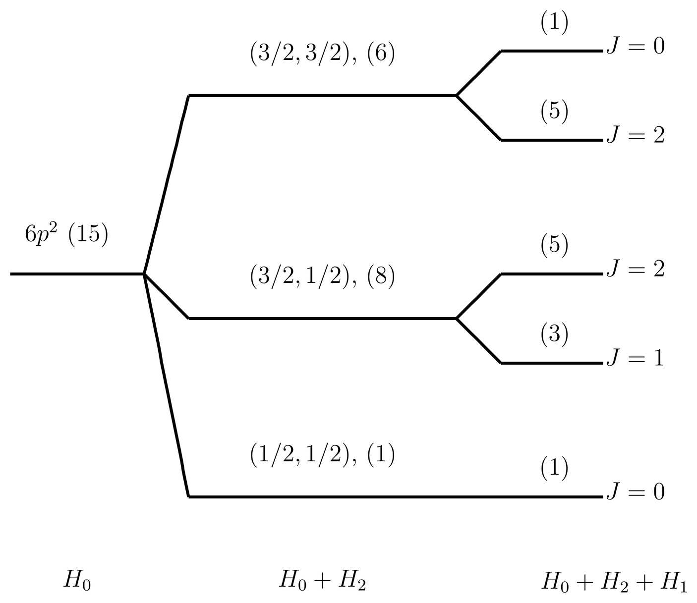
Figure 2:Term diagram in -coupling for lead (Pb). Drawing is not to scale.
Finally, when we turn on , the individual operators no longer commute with the Hamiltonian, but does. Therefore we must now organize the energy eigenstates according to the quantum numbers. In Pb, for example, the state splits into and states. The state , which occurs in , is not allowed by the Pauli principle. Likewise, the level splits into and levels, because . Here the Pauli principle causes no extra restriction, because . Finally, the gives only a level. All these levels and their degeneracies (in parentheses) are indicated in the figure.
(a) For the case of bismuth ( configuration), indicate the allowed terms and their degeneracies when is added to . Make sure the degeneracies add up to the degeneracy of the configuration. Indicate also the allowed values contained in each term.
Problem (b).
The term contains a component. Find the normalized states in this component for and . Write your answers as linear combinations of Slater determinants composed of orbitals ; the Slater determinant will be identified by the quantum numbers of the last three orbitals, since the orbitals for the 80 core electrons are fixed. To help the grader(s), identify these Slater determinants as .