52. Electromagnetic Interactions With the Dirac Field

Introduction¶

In the previous set of notes we second-quantized the Dirac equation for a free particle, and using ideas from hole theory we created a field theory of free electrons and positrons. Notable elements of this procedure were the use of anticommuting creation and annihilation operators and the redefinition of the vacuum to be the state corresponding to the filled Dirac sea in first quantized hole theory. In this set of notes we solve some problems involving the interaction of the second quantized Dirac field with an electromagnetic field. In the first application we adopt a model in which the electromagnetic field is just a given $c$ -number field interacting with the quantized Dirac field; this allows us to find the cross for a relativistic version of Rutherford scattering, called Mott scattering. In a second application our model takes both the electromagnetic field and the Dirac field to be quantized, giving us a theory of electrons, positrons and photons. We use this to find the cross for $e^+$ - $e^-$ annihilation. In the process of working through these examples we develop several computational techniques that are useful for similar problems in quantum electrodynamics. In these notes we continue with natural units, in which $\hbar=c=1$ .

The Dirac Field Interacting With an External Electromagnetic Field¶

The Dirac Lagrangian density for the free field was given by (23), which we reproduce here with a slight change of notation,

{\cal L}_0 = \psibar(i\gamma^\mu\partial_\mu -m)\psi =\psibar(i\partialslash-m)\psi,

(1)

where the 0-subscript means “free particle.” Note that $i\partialslash=i\gamma^\mu\partial_\mu$ can also be written $\pslash$ , if $p_\mu$ is interpreted as the 4-momentum operator $i\partial_\mu$ of the first quantized Dirac theory. To incorporate interactions with the electromagnetic field, we introduce the vector potential $A_\mu(x)$ , assumed to be a given function of $x=(\xvec,t)$ . We assume that the interaction between the Dirac field and the electromagnetic field is given by the minimal coupling prescription, which in the present context means making the replacement

i\partial_\mu \to i\partial_\mu - qA_\mu.

(2)

It is a guess that this gives us the correct interaction between the Dirac field and the electromagnetic field, but as we have seen minimal coupling works well in the first quantized Dirac theory of the electron. Minimal coupling causes the Lagrangian density ${\cal L}_0$ to be replaced by

{\cal L} = {\cal L}_0 + {\cal L}_1,

(3)

where the interaction Lagrangian is given by

{\cal L}_1 = -q\,\psibar \gamma^\mu A_\mu \psi =-q\,\psibar\Aslash\psi= -J^\mu A_\mu,

(4)

where $J^\mu = q\psibar\gamma^\mu\psi$ is the charge current in the Dirac theory.

Altogether, the Lagrangian density is

{\cal L} = \psibar(i\partialslash - q\Aslash -m)\psi.

(5)

Regarded as a classical Lagrangian density for the “classical” fields $\psi$ and $\psibar$ , this gives the Euler-Lagrange equation,

(i\partialslash -q\Aslash -m)\psi=0,

(6)

which is the first quantized Dirac equation for a particle interacting with an external electromagnetic field. See (13) and the derivation of (25). From the Lagrangian density we compute the Hamiltonian density as in The “Classical” Hamiltonian for the Dirac Field, Revisited, finding

{\cal H} = {\cal H}_0 + {\cal H}_1,

(7)

where ${\cal H}_0$ , the free particle Hamiltonian density, is

{\cal H}_0 = \psibar(-i\gammavec\cdot\del + m)\psi =\psi^\dagger(-i\alphavec\cdot\del + m\beta)\psi,

(8)

as in (36), and where the interaction Hamiltonian density is

{\cal H}_1 = -{\cal L}_1 = q\,\psibar\gamma^\mu A_\mu\psi.

(9)

This is all at the “classical” or first quantized level.

To second-quantize the electron-positron field we interpret $\psi$ and $\psibar$ (but not $A_\mu$ ) as field operators and normal order. Then the Hamiltonian is

H = \int d^3\xvec \, ({\cal H}_0 + {\cal H}_1) = H_0 + H_1,

(10)

where

H_0 = \int d^3\xvec \; \mathcolon\psi^\dagger(-i\alphavec\cdot\del +m\beta)\psi\mathcolon = \sum_{ps} E_p (b^\dagger_{ps} b_{ps} + d^\dagger_{ps}d_{ps}),

(11)

exactly as in (85), and where

H_1 = q\int d^3\xvec \; \mathcolon\psibar\gamma^\mu A_\mu\psi\mathcolon.

(12)

We will apply perturbation theory to this Hamiltonian, with the free particle part $H_0$ serving as the unperturbed system.

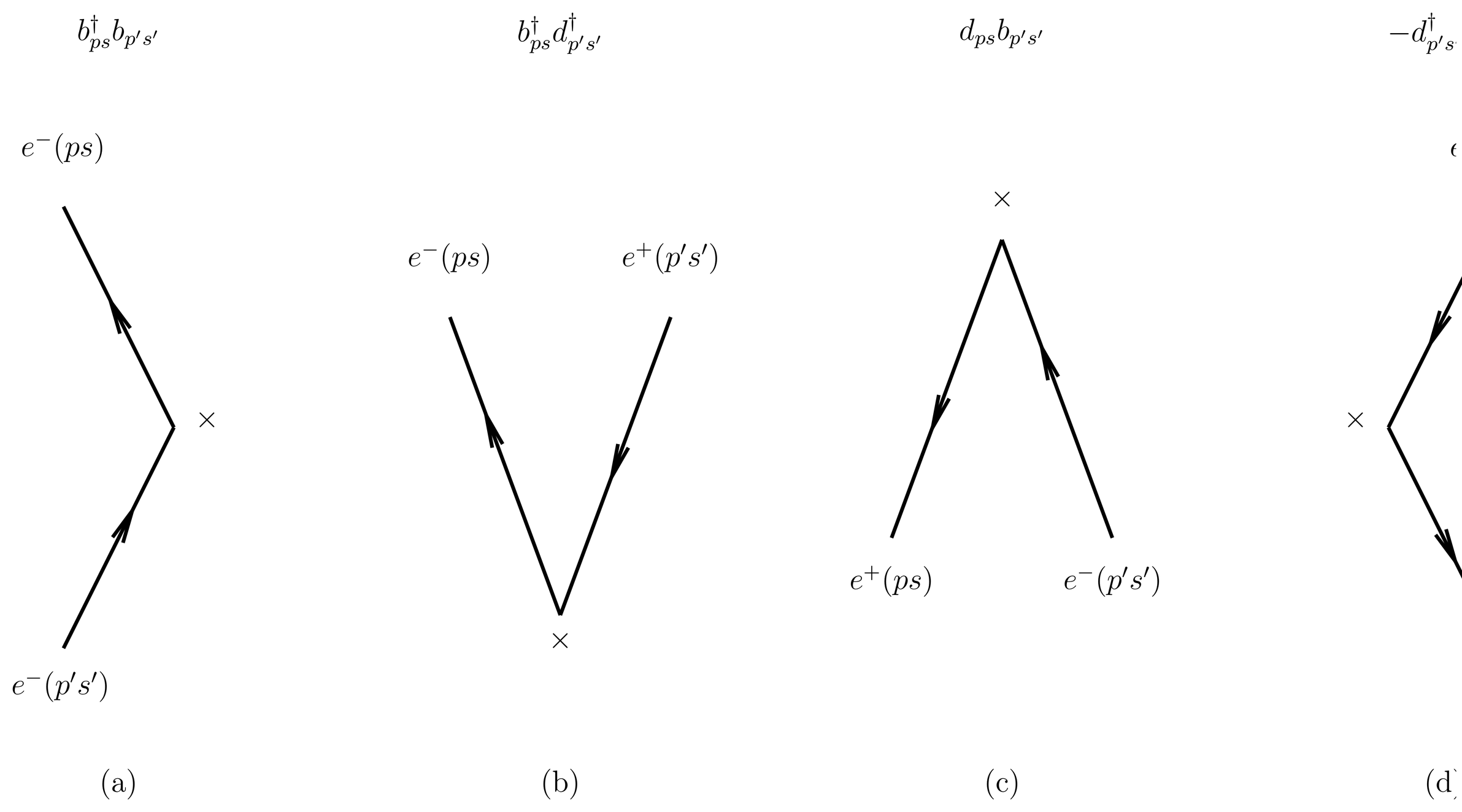
Feynman diagrams for the interaction of the electron-positron field with an external electromagnetic field. The external field is indicated by \cross. Notice the minus sign on diagram (d), arising from the normal ordering. — Figure 1:Feynman diagrams for the interaction of the electron-positron field with an external electromagnetic field. The external field is indicated by $\cross$ . Notice the minus sign on diagram (d), arising from the normal ordering.

Let us look at the processes engendered by $H_1$ in first order perturbation theory. The relevant matrix element is $\matrixelement{b}{H_1}{a}$ , where $\ket{a}$ and $\ket{b}$ are two states. The same matrix element appears in higher order perturbation theory. It has the structure

\matrixelement{b}{H_1}{a} \sim \int d^3\xvec \, \bra{n} \mathcolon\sum_{ps} (b^\dagger_{ps} \ldots d_{ps}) \,\gamma^\mu A_\mu(\xvec,t) \sum_{p's'}( b_{p's'} \ldots d^\dagger_{p's'})\mathcolon\ket{i},

(13)

where we use (81) and (82) and where we omit all normalization constants, etc., and concentrate just on the creation and annihilation operators. There are four combinations of creation and annihilation operators that occur in $H_1$ , corresponding to the four types of Feynman diagrams illustrated in Figure 1. As in 43. Scattering of Radiation by Matter, the Feynman diagrams are basically space-time diagrams, with time increasing from bottom to top.

At the top of the figure is the product of creation and annihilation operators corresponding to the diagram below it. Note the minus sign in part~(d) of the figure, which is due to the normal ordering. Part~(a) of the figure is the scattering of an electron; part~(b) is electron-positron pair creation; part~(c) is pair annihilation; and part~(d) is the scattering of a positron, all taking place in the external field. The interaction with the external field is marked with the symbol $\cross$ . Note that all four diagrams are topologically identical, and just differ by their orientations in space-time. By convention the arrows on the electron lines point in the direction of increasing time, while those on positron lines point backwards in time. This follows the ideas of St"uckelberg and Feynman in which a positron is, in a sense, an electron traveling backwards in time. This convention makes the arrows flow continuously in the same direction along a particle line, even when an electron and positron are created or are annihilated.

Scattering by an External Potential $\Phi(\xvec)$ ¶

Let us now consider scattering of an electron by an external electrostatic potential, $\Phi(\xvec)$ . This is a model, for example, of scattering by an atomic nucleus. Thus we take

A^\mu=(\Phi,\zerovec) \qquad and \qquad \Aslash=\gamma^\mu A_\mu = \gamma^0 \Phi(\xvec).

(14)

We let the incident electron have mode $(ps)$ and the scattered electron have mode $(p's')$ , so the initial and final states are

\ket{i}=b^\dagger_{ps}\ket{0}, \qquad \ket{n}=b^\dagger_{p's'}\ket{0}.

(15)

We set $q=-e$ for the charge of the electron. Then the matrix element appearing in first-order time-dependent perturbation theory is

\begin{aligned} M&=\matrixelement{n}{H_1}{i} = \matrixelement{0}{b_{p's'} H_1 b^\dagger_{ps}}{0} \\ &= -{e\over V} \int d^3\xvec\,\bra{0}b_{p's'}\mathcolon \sum_{p_1s_1} \sqrt{{m\over E_1}} \bigl(b^\dagger_{p_1s_1} \ubar_{p_1s_1}e^{-i\pvec_1\cdot\xvec} +d_{p_1s_1}\vbar_{p_1s_1}e^{i\pvec_1\cdot\xvec}\bigr) \\ &\times \gamma^0\Phi(\xvec) \sum_{p_2s_2}\sqrt{{m\over E_2}}\bigl( b_{p_2s_2} u_{p_2s_2}e^{i\pvec_2\cdot\xvec} + d^\dagger_{p_2s_2}v_{p_2s_2}e^{-i\pvec_2\cdot\xvec} \bigr)\mathcolon b^\dagger_{ps}\ket{0}, \\ \end{aligned}

(16)

where we have used the Fourier series (81) and (82) for $\psi(\xvec)$ and $\psibar(\xvec)$ , and where we have been careful to use dummy variables of summation $(p_1s_1)$ and $(p_2s_2)$ so as to avoid confusion with the initial and final electron modes $(ps)$ and $(p's')$ . Notice that (16) contains an implied multiplication of a row spinor ( $\ubar_{p_1s_1}$ or $\vbar_{p_1s_1}$ ) times a Dirac matrix ( $\gamma^0$ ) times a column spinor ( $u_{p_2s_2}$ or $v_{p_2s_2}$ ).

Because of the anticommutation relations among the creation and annihilation operators, the only term from the two Fourier series that survives is the $b^\dagger b$ term with $(p_1s_1)=(p's')$ and $(p_2s_2)=(ps)$ . That is, when we evaluate the field part of the matrix element (16), we get

\matrixelement{0}{b_{p's'} b^\dagger_{p_1s_1} b_{p_2s_2} b^\dagger_{ps}}{0} = \delta_{pp_2}\,\delta_{ss_2}\, \matrixelement{0}{b_{p's'} b^\dagger_{p_1s_1}}{0} =\delta_{pp_2}\,\delta_{ss_2}\,\delta_{p'p_1}\,\delta_{s's_1},

(17)

where we have used the anticommutation relations (53) to migrate annihilation operators $b$ toward the vacuum ket on the right, which they annihilate. All other terms such as the one in $b^\dagger d^\dagger$ give zero, so that only the electron scattering diagram (a) in Figure 1 contributes. Thus we find

\begin{aligned} M=&-{e\over V} \int d^3\xvec \, \sqrt{{m^2\over EE'}} \bigl(\ubar_{p's'}\gamma^0 u_{ps}\bigr) \, e^{-i(\pvec'-\pvec)\cdot\xvec}\, \Phi(\xvec) \\ &=-{e\over V}(2\pi)^{3/2} \, \sqrt{{m^2\over EE'}}\, \tilde\Phi(\qvec) \bigl(\ubar_{p's'}\gamma^0 u_{ps}\bigr), \\ \end{aligned}

(18)

where we use the convention (83) for the Fourier transform $\tilde\Phi$ of $\Phi$ and where $\qvec=\pvec'-\pvec$ is the momentum transfer.

According to first-order time-dependent perturbation theory, the probability $P_n$ of the system being in final state $\ket{n}$ is

P_n(t)= {2\pi t}\,\Delta_t(\omega_{ni}) |\matrixelement{n}{H_1}{i}|^2,

(19)

where $n$ , the general notation for the final state, is identified with $(p's')$ in our application. To compute the differential cross $d\sigma/d\Omega'$ , where $\Omega'$ refers to the direction of the scattered electron, we must sum over all final states $(p's')$ such that $\pvec'$ lies in a small cone of solid angle $d\Omega'$ centered on some direction $(\theta',\phi')$ . We must also divide by the time to get the transition rate, and by the incident flux, which is

J_inc = {v\over V} = {p_3\over EV},

(20)

where $v$ , $p_3=|\pvec|$ and $E$ are the velocity, momentum and energy of the incident electron. Because of box normalization, there is one incident electron in the box of volume $V$ , so that the density of incident particles is $1/V$ . We write $p_3$ for the magnitude of the incident 3-momentum $\pvec$ since we are using the symbol $p=(E,\pvec)$ for the 4-momentum. The initial and final energies are $E$ and $E'$ , so $\omega_{ni}$ in (20) is identified with $E'-E$ .

We follow the usual procedures in time-dependent perturbation theory, including replacing $\Delta_t(\omega_{ni})$ by $\delta(E-E')$ , and making the replacement,

\sum_{\pvec'\in\,cone} \to {V\over (2\pi)^3} \int_cone d^3\pvec' = {V\over (2\pi)^3} \Delta\Omega' \int_0^\infty p_3^{\prime\,2}\, dp'_3,

(21)

where $p'_3=|\pvec'|$ is the magnitude of the final 3-momentum, not to be confused with the final 4-momentum $p'=(E',\pvec')$ . Then

{d\sigma\over d\Omega'} = {EV\over p_3} {V\over (2\pi)^3} \int_0^\infty p_3^{\prime\,2} \,dp'_3 \, 2\pi\,\delta(E'-E) \, |M|^2.

(22)

Now using the rules of $\delta$ -functions we can write

\delta(E'-E) = {E'\over p'_3}\delta(p'_3-p_3),

(23)

and using (18) for $M$ we obtain finally

{d\sigma\over d\Omega'} = 2\pi e^2 m^2 |\tilde\Phi(\qvec)|^2 |\ubar_{p's'}\gamma^0 u_{ps}|^2.

(24)

Note that the $\delta$ -function forces $p'_3=p_3$ and therefore $E'=E$ , so that after the integral has been done the initial and final 4-momenta become

p=(E,\pvec), \qquad p'=(E,\pvec'),

(25)

that is, with the same energy.

Summing and Averaging over Spin States¶

The differential cross (22) depends the energy $E$ of the incident momentum, the directions of the initial and final momenta $\pvec$ and $\pvec'$ , and the spins $s$ and $s'$ of the initial and final electron states. Recall that in the nonrelativistic (electrostatic) limit the scattering cross is independent of the spin. (See (86), in which $\tilde U$ can be replaced by $-e\tilde\Phi$ to compare with (22).)

In many applications the initial electron beam is unpolarized and we do not care about the spin of the scattered electron. Then the effective cross is obtained by averaging over initial spin states and summing over final spin states. This means that we must make the replacement,

|\ubar_{p's'}\gamma^0 u_{ps}|^2 \to {1\over2} \sum_{ss'} |\ubar_{p's'}\gamma^0 u_{ps}|^2.

(26)

Spin sums of this type are very common in problems involving relativistic electrons, so we will now illustrate some techniques that are useful in evaluating them.

First we write

{1\over2}\sum_{ss'} |\ubar_{p's'}\gamma^0 u_{ps}|^2 = {1\over 2} \sum_{ss'} (\ubar_{p's'}\gamma^0 u_{ps}) (\ubar_{ps} \gamma^0 u_{p's'}).

(27)

This result would be more obvious if the second factor were written

(\ubar_{p's'}\gamma^0 u_{ps})^\cc,

(28)

but in fact they are the same, since the expression (28) can be written

(u^\dagger_{p's'}\gamma^0 \gamma^0 u_{ps})^\cc = u^\dagger_{ps} \gamma^0 \gamma^0 u_{p's'} = \ubar_{p's'}\gamma^0 u_{p's'},

(29)

since $\gamma^0$ is Hermitian. Now the sum (27) can be written as a trace,

{1\over2}\tr\Bigl[\gamma^0 \Bigl(\sum_s u_{ps}\ubar_{ps}\Bigr) \gamma^0 \Bigl(\sum_{s'} u_{p's'}\ubar_{p's'}\Bigr)\Bigr],

(30)

in which the sums are positive energy projectors $\Pi_+$ , as indicated by (153). Then we can use (39) to write the spin sum as

{1\over2}\tr\Bigl[\gamma^0 \Bigl({m+\pslash\over 2m}\Bigr) \gamma^0 \Bigl({m+\pslash^{\,\prime}\over 2m}\Bigr)\Bigr].

(31)

In this manner, the spin sum has been transformed into the trace of a polynomial in the $\gamma$ matrices.

Traces of Products of $\gamma$ -Matrices¶

We now present some rules for evaluating the traces of products of $\gamma$ -matrices. The rules we will use are

\begin{aligned} \tr 1 &= 4, \end{aligned}

(32)

\begin{aligned} \tr(\gamma^\mu\gamma^\nu) &= 4g^{\mu\nu}, \end{aligned}

(33)

\begin{aligned} \tr(\gamma^\mu\gamma^\nu\gamma^\alpha\gamma^\beta)&= 4(g^{\mu\nu}g^{\alpha\beta} - g^{\mu\alpha}g^{\nu\beta} +g^{\mu\beta}g^{\nu\alpha}), \end{aligned}

(34)

\begin{aligned} \tr(\\textany odd number of \gamma's) &=0. \end{aligned}

(35)

Alternative versions of rules (33) and(34) are

\begin{aligned} \tr(\aslash\bslash) &= 4(a\cdot b), \end{aligned}

(36)

\begin{aligned} \tr(\aslash\bslash\cslash\dslash) &= 4[(a\cdot b)(c\cdot d) - (a\cdot c)(b\cdot d) + (a\cdot d)(b\cdot c)], \end{aligned}

(37)

where we use the notation $(a\cdot b)=a_\mu b^\mu$ for the scalar product of two 4-vectors, as in (104).

Now we present the proofs of these formulas. The proof of (32) is trivial. We prove (33) with the help of the fundamental anticommutation relation (18),

\tr(\gamma^\mu\gamma^\nu) = 2g^{\mu\nu} \tr(1) - \tr(\gamma^\nu\gamma^\mu).

(38)

But by cycling the products in the final trace, it becomes equal to the trace on the left-hand side. Using (32) we then obtain (33).

The proof of (34) is similar but more elaborate. We use the fundamental anticommutation relation (18) to migrate $\gamma^\mu$ to the right in three steps, obtaining

\tr(\gamma^\mu\gamma^\nu\gamma^\alpha\gamma^\beta) = 2g^{\mu\nu}\tr(\gamma^\alpha\gamma^\beta) - 2g^{\mu\alpha}\tr(\gamma^\nu\gamma^\beta) + 2g^{\mu\beta}\tr(\gamma^\nu\gamma^\alpha) - \tr(\gamma^\nu\gamma^\alpha\gamma^\beta\gamma^\mu),

(39)

whereupon by cycling the factors in the final trace it becomes equal to the left-hand side. Then with the aid of (33) we derive (34). It is clear that with techniques like this the trace of the product of any even number $n$ of $\gamma$ -matrices can be reduced sums of traces of products of $n-2$ $\gamma$ -matrices.

The proof of (35) uses the properties of the matrix $\gamma_5=i\gamma^0\gamma^1\gamma^2\gamma^3$ , namely, $\gamma_5^2=1$ and $\{\gamma_5,\gamma^\mu\}=0$ (see (109). For example, in the case of the trace of the product of three $\gamma$ -matrices we have

\begin{aligned} \tr(\gamma^\mu\gamma^\nu\gamma^\alpha) &= \tr(\gamma_5^2\gamma^\mu\gamma^\nu\gamma^\alpha) = -\tr(\gamma_5\gamma^\mu\gamma^\nu\gamma^\alpha\gamma_5) =-\tr(\gamma_5^2\gamma^\mu\gamma^\nu\gamma^\alpha) \\ &=-\tr(\gamma^\mu\gamma^\nu\gamma^\alpha)=0, \\ \end{aligned}

(40)

where in the second equality we have migrated one of the $\gamma_5$ ’s past the three other $\gamma$ -matrices, incurring three minus signs, and in the third we have cycled the factors, restoring the original trace but with a minus sign. This procedure obviously works for any odd number of $\gamma$ -matrices.

The Mott Cross Section¶

Now we may evaluate the trace (31). Multiplying the factors out and dropping terms that are of odd order in $\gamma^\mu$ , the expression (31) becomes

{1\over 8m^2}\tr\bigl( m^2 \gamma^0\gamma^0 + \gamma^0\pslash\gamma^0\pslash^{\,\prime}\bigr) = {1\over 2m^2}\bigl(m^2 g^{00} + 2EE' - g^{00}(p\cdot p') \bigr).

(41)

But $g^{00}=1$ , $p\cdot p'=EE'-\pvec\cdot\pvec'$ , $E=E'$ , and $m^2=E^2-|\pvec|^2$ , so this expression becomes

{1\over 2m^2}(2E^2 - |\pvec|^2 + \pvec\cdot\pvec') ={1\over 2m^2}[2E^2 - |\pvec|^2(1-\cos\theta)],

(42)

where we have used $|\pvec|=|\pvec'|$ and where $\theta$ is the angle between $\pvec$ and $\pvec'$ , that is, it is the scattering angle. This can also be written

{1\over m^2} [E^2-|\pvec|^2\sin^2(\theta/2)] = {E^2\over m^2}[1-v^2\sin^2(\theta/2)],

(43)

where $v=|\pvec|/E$ is the velocity of the incident electron.

Now we can make the replacement (26) in the cross (24), obtaining,

{d\sigma\over d\Omega'} = 2\pi\,e^2E^2|\tilde\Phi(\qvec)|^2 [1-v^2\sin^2(\theta/2)].

(44)

If the potential $\Phi(\xvec)$ arises from an extended charge distribution, for example, the interior of a proton or a nucleus, then the method of form factors can be used, as discussed in Application: Electrostatic Scattering and Form Factors. But in the case of scattering by a point charge $Ze$ , for which the potential is $\Phi(\xvec)=-Ze^2/|\xvec|$ , the Fourier transform of the potential is

\tilde\Phi(\qvec) = -{2Ze^2\over \sqrt{2\pi}}\, {1\over q^2}.

(45)

A direct evaluation of the Fourier transform of the Coulomb potential is tricky because of the singularity, but by multiplying the potential by $e^{-\kappa r}$ it becomes a Yukawa potential whose Fourier transform is easier to evaluate, and which is given in (127). Taking the limit $\kappa\to0$ then gives (45). Also, the square of the 3-momentum transfer can be written,

q^2 = 2|\pvec|^2(1-\cos\theta) = 4|\pvec|^2\sin^2(\theta/2),

(46)

so that altogether we obtain the cross for the scattering of relativistic electrons by a positive point charge,

{d\sigma\over d\Omega'} = {Z^2e^4 E^2 \over 4p^4 \sin^4(\theta/2)}[1-v^2\sin^2(\theta/2)],

(47)

where we now just write $p$ for the magnitude of the 3-momentum $\pvec$ . This is a relativistic version of the Rutherford cross , given by (119); in comparing the two, it should be noted that $E$ in the nonrelativistic formula is $p^2/2m$ , whereas in (47) it is the relativistic energy, $(m^2+p^2)^{1/2}$ , and that moreover the relativistic formula is expressed in units in which $\hbar=c=1$ . Formula (47) is called the *Mott cross *. The correction factor $v^2\sin^2(\theta/2)$ comes from the spin of the electron; it is absent in the scattering of charged particles of spin~0. It obviously becomes important at large scattering angles ( $\theta\to\pi$ ) and at high velocities ( $v \to 1$ , in the formula; $v\to c$ in ordinary units). As $v\to c$ , magnetic forces become as important as electric forces, which is what we see here.

Covariant Lagrangian for the Interacting Dirac and Electromagnetic Fields¶

Now we turn to problems that involve the second-quantized Dirac field and the quantized electromagnetic field, that is, problems with electrons, positrons and photons.

We begin at the “classical” level at which this system is the first-quantized Dirac field interacting with a classical or $c$ -number electromagnetic field. The classical Lagrangian density is

{\cal L}={\cal L}_D + {\cal L}_em + {\cal L}_int,

(48)

where ${\cal L}_D$ is the free Dirac Lagrangian density,

{\cal L}_D = \psibar(i\partialslash -m)\psi

(49)

(see (23), where ${\cal L}_em$ is the Lagrangian density for the free electromagnetic field,

{\cal L}_em={1\over 16\pi} F^{\mu\nu}F_{\nu\mu} ={1\over 8\pi}(E^2-B^2)

(50)

(see (13), and where ${\cal L}_int$ is the interaction Lagrangian density,

{\cal L}_int =-J^\mu A_\mu

(51)

(see (19). This is a combination of the Lagrangian density for the electromagnetic field driven by a matter current $J^\mu$ , as in The Electromagnetic Lagrangian, and the Lagrangian density (5) for the “classical” Dirac field driven by an external electromagnetic field via minimal coupling. Note that the current is given by

J^\mu = -e\psibar \gamma^\mu \psi,

(52)

so that

{\cal L}_int = e\psibar \Aslash \psi,

(53)

where we set $q=-e$ for the electron.

If $A^\mu$ (all four components), $\psi$ and $\psibar$ are regarded as independent fields, then the Euler-Lagrange equations arising from the Lagrangian density (48) are

\begin{aligned} (i\partialslash -m)\psi &= -e\Aslash\psi, \end{aligned}

(54)

\begin{aligned} \partial_\nu F^{\nu\mu} &= 4\pi J^\mu, \end{aligned}

(55)

that is, they are the first quantized Dirac equation driven by the electromagnetic field, and Maxwell’s equations, driven by the Dirac charge current. Here we present Maxwell’s equations in covariant form, see (95), because we wish to emphasize that that the equations of motion, taken as a whole, are covariant. But (55) is equivalent to the $(3+1)$ -version of Maxwell’s equations, (21).

Coulomb Gauge and Covariant Quantization¶

In preparation for quantization of this system we now introduce Coulomb gauge, which breaks both gauge invariance and manifest Lorentz covariance. This means that the intermediate steps in our subsequent calculations will not be Lorentz covariant, although the final answers will be, since the theory itself is Lorentz covariant and a choice of gauge is just a convention that drops out when physical answers are derived.

As pointed out in 40. The Classical Electromagnetic Field Hamiltonian{} and shown in detail in 42. Emission and Absorption of Radiation, one of the advantages of Coulomb gauge is that it gives good unperturbed Hamiltonians for the interaction of matter with radiation when the matter is essentially nonrelativistic and all velocities are small compared to the speed of light. In the applications we are about to consider, however, we will be dealing with problems in which the particles may take on relativistic velocities, and ones in which particles are created and/or destroyed. Therefore this would be a good point to switch over to completely covariant methods, were it not for the extra formalism required to do so. Nevertheless, we will say a few words about what is involved in covariant quantization.

The quantization of the Dirac field outlined in 51. Hole Theory and Second Quantization of the Dirac Equation{} is already fully covariant, but that of the electromagnetic field, carried out in Coulomb gauge in 41. The Quantized Electromagnetic Field, is not. The electromagnetic field is a gauge field with nonphysical gauge degrees of freedom. These are associated with “constraints,” that is, algebraic relations among the field variables that are not evolution equations. The principal constraint in electromagnetism is Gauss’s law, $\del\cdot\Evec=4\pi\rho$ , which ties the longitudinal component of the electric field to the matter degrees of freedom. It is not an evolution equation. There are fully covariant ways of quantizing the electromagnetic field, but they involve the introduction of new degrees of freedom, corresponding to “longitudinal” and “scalar” photons. Photons that correspond to actual light waves are always transverse, and these are the only ones that we see in Coulomb gauge. But in a covariant quantization, the longitudinal and scalar photons appear when describing electromagnetic fields that do not propagate, such as electrostatic fields, and they also appear in a covariant description of intermediate states in perturbation theory, that is, as virtual photons.

Moreover, the version of perturbation theory that we have been using, which is sometimes called “old fashioned perturbation theory,” is not covariant. Covariant perturbation theory exists, but it is another piece of formalism we would have to master before turning to a fully covariant treatment of the interaction of the Dirac field with the electromagnetic field.

We shall proceed with Coulomb gauge and noncovariant perturbation theory. It is not wrong, and it is not too bad for the problems we shall consider. You will be able to see how the results we obtain can be assembled into covariant answers, and it how the pieces of noncovariant perturbation theory can be assembled into their fully covariant versions.

Coulomb Gauge in the “Classical” Theory¶

Recall that in Coulomb gauge the scalar potential $\Phi$ is not an independent variable, but rather it is determined by the charge density via Coulomb’s law. That is,

\Phi(\xvec) = \int d^3\xvec' {\rho(\xvec')\over |\xvec-\xvec'|},

(56)

where in the present context the charge density is that of the Dirac electron,

\rho(\xvec)=-e\psi^\dagger(\xvec)\psi(\xvec).

(57)

Recall also that the fields in (56) are evaluated at the same time, that is, $\Phi$ is the nonretarded potential. Also, the vector potential $\Avec$ is purely transverse, so its longitudinal component vanishes, and the longitudinal and transverse parts of the electric field are

\Evec_\parallel = -\del\Phi, \qquad \Evec_\perp = -\frac{\partial \Avec}{\partial t}.

(58)

In Coulomb gauge it is convenient to transform the Lagrangian, the spatial integral of the Lagrangian density (48). Ignoring the Dirac part of the Lagrangian for the moment, we have

L_em + L_int = \int d^3\xvec\, \Bigl[{1\over 8\pi}(E^2-B^2) -\rho\Phi + \Jvec\cdot\Avec\Bigr],

(59)

where $\rho$ is given by (57). First we note that

\int d^3\xvec\, E^2 = \int d^3\xvec\, (\Evec_\parallel + \Evec_\perp)^2 = \int d^3\xvec\, (E_\parallel^2 + E_\perp^2),

(60)

since the cross terms involving $\Evec_\parallel\cdot\Evec_\perp$ vanish when integrated over all space (see (31). As for the longitudinal electric field energy, it can be transformed as in The Hamiltonian for the Matter-Field System,

{1\over 8\pi}\int d^3\xvec\, E_\parallel^2 = {1\over 8\pi}\int d^3\xvec\, (\del\Phi)^2 = {1\over 8\pi} \int d^3\xvec\, [\del\cdot(\Phi\del\Phi) - \Phi\del^2\Phi] = {1\over 2} \int d^3\xvec\, \Phi\rho,

(61)

where we drop boundary terms and use $\del^2\Phi=-4\pi\rho$ (valid in Coulomb gauge). The final expression cancels one half of the term $-\rho\Phi$ in the Lagrangian (59), so that overall the Lagrangian (including now the Dirac term) is

L = \int d^3\xvec\, \Bigl[ {1\over 8\pi}(E_\perp^2-B^2) -{1\over2}\rho\Phi + \Jvec\cdot\Avec + \psibar(i\partialslash-m)\psi\Bigr].

(62)

The independent fields in this Lagrangian are the transverse components of $\Avec$ (which has no longitudinal component), and $\psi$ and $\psibar$ . The scalar potential $\Phi$ depends on $\psi$ and $\psibar$ through (56)--(57), and is not independent. It can be shown that when the action $S=\int L\,dt$ is forced to be stationary with respect to variations in these independent fields, the result is the equations of motion (54). The derivation is slightly tricky, and is relegated to Prob.~\prbremdirac-1.

We can now derive the Hamiltonian from the Lagrangian (62). The momentum conjugate to $\psi$ is

\pi=\pop{{\cal L}}{\dot{\psi}}= \psibar (i\gamma^0),

(63)

as in (34), while the momentum $\bar\pi$ conjugate to $\psibar$ vanishes. The momentum conjugate to $\Avec$ is

\Pvec=\pop{{\cal L}}{\dot\Avec} = -{\Evec_\perp\over 4\pi},

(64)

where it is understood that $\Evec_\perp$ is an abbreviation for $-\dot\Avec$ in the Lagrangian (62). Altogether, then, the Hamiltonian density is

{\cal H} = \psibar\Bigl(i\gamma^0\frac{\partial \psi}{\partial t}\Bigr) + \Pvec\cdot\dot\Avec - {\cal L} ={\cal H}_D + {\cal H}_em + {\cal H}_\text{Coul} +{\cal H}_T,

(65)

where

\begin{aligned} {\cal H}_D &= \psibar\bigl(-i\gammavec\cdot\del +m\bigr)\psi = \psi^\dagger\bigl(-i\alphavec\cdot\del + m\beta\bigr)\psi, \end{aligned}

(66)

\begin{aligned} {\cal H}_{em} &= {E_\perp^2 + B^2\over 8\pi}, \end{aligned}

(67)

\begin{aligned} {\cal H}_\text{Coul} &= {1\over 2} \rho\Phi, \end{aligned}

(68)

\begin{aligned} {\cal H}_T &= -\Jvec\cdot\Avec = e\psibar \gammavec\cdot\Avec\psi = e\psi^\dagger\alphavec\cdot\Avec\psi, \end{aligned}

(69)

and where the $T$ on ${\cal H}_T$ stands for “transverse.”

The Quantum System¶

We quantize the system by interpreting the fields $\psi$ , $\psibar$ and $\Avec$ as quantum fields with the Fourier expansions (81), (82) and (22), respectively. All three of these employ box normalization in a box of volume $V$ . For reference we write out the last of these in natural units ( $\hbar=c=1)$ :

\Avec(\xvec)=\sqrt{{2\pi\over V}} \sum_\lambda {1\over\sqrt{\omega}}[a_\lambda {\hat{\boldsymbol{\epsilon}}}_\lambda \,e^{i\kvec\cdot\xvec} + a^\dagger_\lambda {\hat{\boldsymbol{\epsilon}}}^\cc_\lambda\,e^{-i\kvec\cdot\xvec}],

(70)

where as usual $\lambda=(\kvec\mu)$ is an abbreviation for the mode of the electromagnetic field. The Hamiltonian is then the spatial integral of the Hamiltonian density, which we must normal order. We write it as $H=H_0+H_1$ , where $H_0=H_D+H_em$ is the free field Hamiltonian,

\begin{aligned} H_D &= \int d^3\xvec \, \mathcolon \psi^\dagger (-i\alphavec\cdot\del + m)\psi\mathcolon = \sum_{ps}E_p(b^\dagger_{ps}b_{ps}+d^\dagger_{ps}d_{ps}), \end{aligned}

(71)

\begin{aligned} H_em&=\int d^3\xvec\, {\mathcolon E_\perp^2 + B^2\mathcolon\over 8\pi} =\sum_\lambda \omega_\lambda\, a^\dagger_\lambda a_\lambda, \end{aligned}

(72)

and where $H_1= H_\text{Coul} + H_T$ is the perturbing Hamiltonian,

\begin{aligned} H_\text{Coul} &= {1\over 2} \int d^3\xvec\, \mathcolon\rho(\xvec)\Phi(\xvec)\mathcolon = {1\over 2} \int d^3\xvec\,d^3\xvec'\, {\mathcolon \rho(\xvec)\rho(\xvec')\mathcolon \over |\xvec-\xvec'|} \end{aligned}

(73)

\begin{aligned} &= {e^2\over 2} \int d^3\xvec\,d^3\xvec'\, {\mathcolon [\psibar(\xvec) \gamma^0 \psi(\xvec)][\psibar(\xvec')\gamma^0\psi(\xvec')] \mathcolon\over |\xvec-\xvec'|}, \end{aligned}

(74)

\begin{aligned} H_T &= -\int d^3\xvec \, \mathcolon\Jvec\cdot\Avec\mathcolon = e\int d^3\xvec\, \mathcolon \psibar(\xvec)\gammavec \cdot\Avec(\xvec)\psi(\xvec)\mathcolon. \end{aligned}

(75)

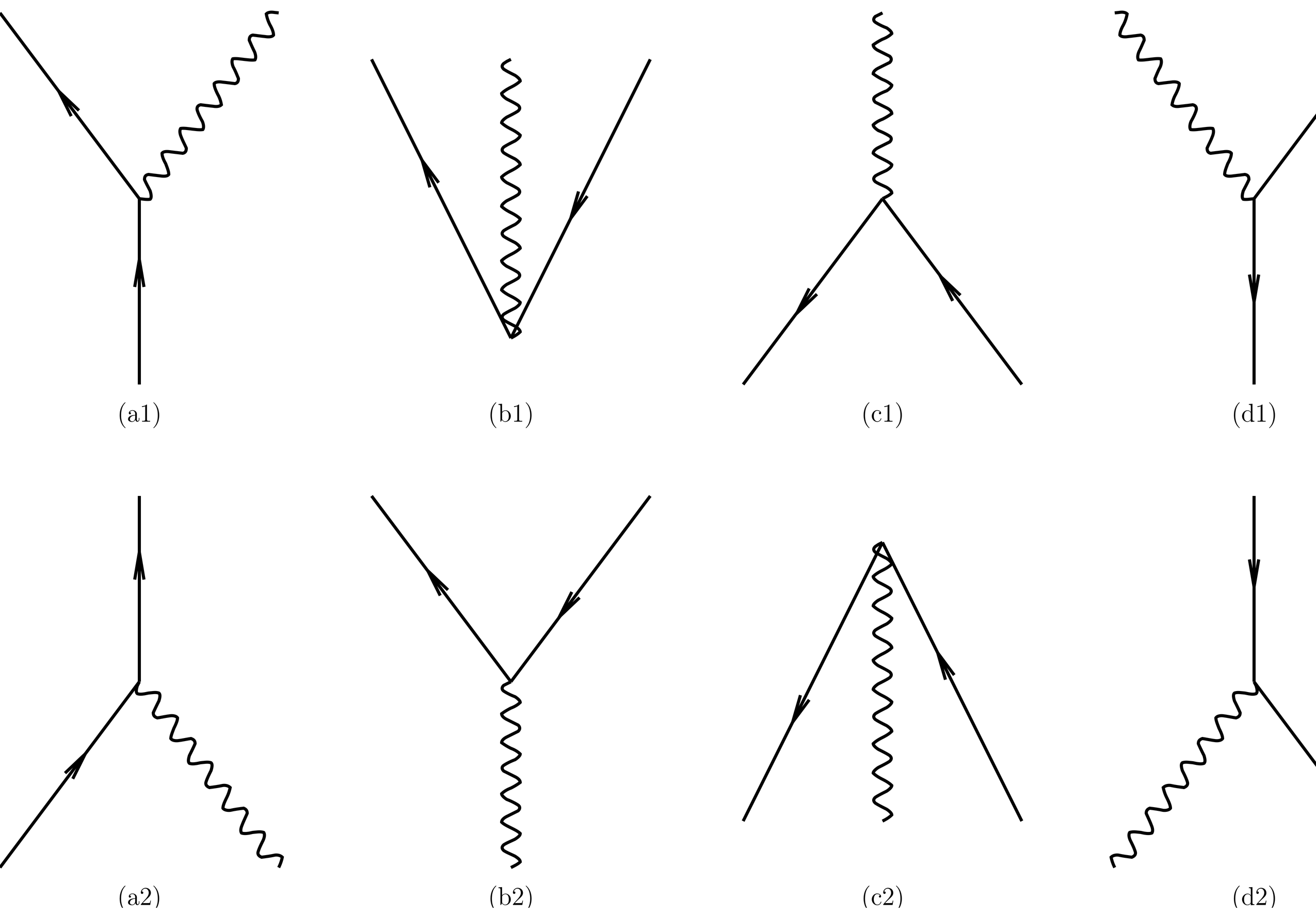
Feynman diagrams generated by H_T. These are the same as in , except for the addition of a photon line, representing either the creation or the destruction of a photon. — Figure 2:Feynman diagrams generated by $H_T$ . These are the same as in Figure 1, except for the addition of a photon line, representing either the creation or the destruction of a photon.

Let us now consider the processes engendered by $H_T$ in first order perturbation theory. For simplicity we treat only $H_T$ and ignore $H_\text{Coul}$ . The matrix element has the structure

\matrixelement{b}{H_1}{a} \sim \int d^3\xvec \, \bra{b} \mathcolon\sum_{ps} (b^\dagger_{ps} \ldots d_{ps}) \,\sum_\lambda(a_\lambda \ldots a^\hc_\lambda)\,\sum_{p's'}( b_{p's'} \ldots d^\dagger_{p's'})\mathcolon\ket{a},

(76)

as in (13) except that now the vector potential $\Avec$ is a quantum field. There are altogether $2^3=8$ combinations of creation and annihilation operators, which produce the Feynman diagram fragments seen in Fig.Figure 2.

Diagrams (a1) and (d1) are the emission of a photon by an electron or positron, while (a2) and (d2) are the absorption of a photon by an electron or positron, respectively. Diagram (b1) is the creation of an electron-positron pair plus a photon out of the vacuum, and (c2) is the annihilation of the same into the vacuum. Finally, diagram (c1) is electron-positron annihilation into a photon, while diagram (b2) is a photon materializing into an electron-positron pair. As in Figure 1, all diagrams are topologically identical, and differ only by the directions in which the lines go in space-time. Note also that in all diagrams, charge is conserved at the vertex. As we will see, in noncovariant perturbation theory, 3-momentum is also conserved at each vertex but not energy, while in covariant perturbation theory, 4-momentum (including energy) is conserved at each vertex.

Electron-Positron Annihilation¶

Now we consider the reaction,

e^- + e^+ \to \gamma\gamma,

(77)

that is, electron-positron annihilation into two photons, as an example of a process involving the Dirac field with multiple particles. Although there is a diagram for the annihilation of an electron and positron into a single photon, (c1) in Figure 2, single-photon annihilation cannot take place in vacuum because it is impossible to satisfy overall energy and momentum conservation. But annihilation into two photons can occur, and we shall now calculate the cross-for the process. We denote the modes of the incident electron and positron by $(ps)$ and $(p's')$ respectively, and of the two photons by $\lambda=(\kvec\mu)$ and $\lambda'=(\kvec'\mu')$ . We will write 4-vectors $p=(E,\pvec)$ and $p'=(E',\pvec')$ for the initial electron and positron, respectively, and 4-vectors $k=(\omega,\kvec)$ and $k'=(\omega',\kvec')$ for the two final photons.

The process (77) cannot happen in first-order perturbation theory, because $H_T$ is capable of creating only a single photon. That is,

\matrixelement{n}{H_T}{i}=0.

(78)

Therefore we will have to take $H_T$ in second order perturbation theory to find a contribution to the process (77). As for $H_\text{Coul}$ , it does not contain any photon creation operators, so it does not contribute and we will ignore it for this calculation.

The transition probability is

P_n = 2\pi t \,\Delta_t(\omega_{ni})\, |M|^2,

(79)

in a general notation in which $\ket{i}$ and $\ket{n}$ are the initial and final states, and where for this problem we have

M=\sum_k {\matrixelement{n}{H_T}{k} \matrixelement{k}{H_T}{i} \over E_i-E_k},

(80)

where $\ket{k}$ is an intermediate state. For this problem we write

\ket{i}=b^\dagger_{ps}d^\dagger_{p's'}\ket{0}, \qquad \ket{n}=a^\dagger_\lambda a^\dagger_{\lambda'}\ket{0}

(81)

so that

\omega_{ni} = \omega+\omega'-E-E'.

(82)

It is important to recognize that the final state is identified by the two modes $\{\lambda,\lambda'\}$ without regard to order, since the photons are identical. That is, the state $(\lambda,\lambda')$ is identical to $(\lambda',\lambda)$ .

The sum over intermediate states in principle runs over a complete set of states of both the electron-positron and the electromagnetic field, including any number of particles. But most terms in this vast sum vanish. To see which terms do contribute, let us write out the structure of the product of matrix elements that appears in (80):

\begin{aligned} &\matrixelement{n}{H_T}{k} \matrixelement{k}{H_T}{i} \\ &\sim \int d^3\xvec\,d^3\xvec' \bra{n}\mathcolon (b^\dagger \ldots d)(a \ldots a^\dagger) (b \ldots d^\dagger)\mathcolon\ket{k} \bra{k}\mathcolon (b^\dagger \ldots d)(a \ldots a^\dagger)(b \ldots d^\dagger) \mathcolon \ket{i}, \\ \end{aligned}

(83)

where the first matrix element contains fields $\psibar\Avec\psi$ evaluated at $\xvec$ , and the second fields $\psibar\Avec\psi$ evaluated at $\xvec'$ .

There are $2^6=64$ combinations of creation and annihilation operators in this, but most of them do not contribute. First of all, the initial state has no photons and the final state has two, so each application of the vector potential $\Avec$ must create a single photon. That is, the terms involving the $a_\lambda$ operators do not contribute, and we keep only the ones involving $a^\dagger_\lambda$ . (Recall that time advances from right to left, taking us from the initial state to the final state.) Next, because we must annihilate the incident $e^-$ , $e^+$ pair in two steps, and because there are a total of four fermion creation or annihilation operators between the initial and final state, we must use three annihilation and one creation operator. Moreover, the pattern must be $AAAC$ or $AACA$ , because, if it were, for example, $CAAA$ , then the intermediate state would contain no fermions, and the third annihilation operator (proceeding from the right) would annihilate it. And if it were $ACAA$ , then normal ordering in $\matrixelement{n}{H_T}{k}$ would convert it to $CAAA$ , with the same effect. The surviving possibilities are summarized in Table 1.

Table 1:Patterns of creation/annihilation operators that contribute to $e^-$ - $e^+$ annihilation.

Case	$\bar{\psi}(x)$	$\Avec(x)$	$\psi(x)$	$\bar{\psi}(x')$	$\Avec(x')$	$\psi(x')$
$1A$	$d_{p' s'}$	$a_{\lambda'}^\dagger$	$b_{p_1 s_1}$	$b_{p_1 s_1}^\dagger$	$a_\lambda^\dagger$	$b_{ps}$
$2A$	$d_{p_2 s_2}$	$a_\lambda^\dagger$	$b_{ps}$	$d_{p' s'}$	$a_{\lambda'}^\dagger$	$d_{p_2 s_2}^\dagger$
$1B$	$d_{p' s'}$	$a_\lambda^\dagger$	$b_{p_1 s_1}$	$b_{p_1 s_1}^\dagger$	$a_{\lambda'}^\dagger$	$b_{ps}$
$2B$	$d_{p_2 s_2}$	$a_{\lambda'}^\dagger$	$b_{ps}$	$d_{p' s'}$	$a_\lambda^\dagger$	$d_{p_2 s_2}^\dagger$

Row $1A$ of the table contains the pattern $AACA$ of fermion operators. Since we are picking the annihilation operator from the final factor $\psi(\xvec')$ it must be an electron annihilation operator; and since the electron we must annihilate is the incident electron, its mode is $(ps)$ , and the operator is $b_{ps}$ , as indicated at the right side of row $1A$ . In the factor $\psibar(\xvec')$ we must pick a creation operator, which must be an electron creation operator; we have denoted its mode by $(p_1s_1)$ in the table, and it is an electron in the intermediate state $\ket{k}$ . There is also a photon creation operator in $\Avec(\xvec')$ ; it must create one of the final photons, which in row $1A$ we arbitrarily choose to be mode $\lambda$ . Thus, in row 1A, the intermediate state contains the incident positron, in mode $(p's')$ ; the intermediate electron, in mode $(p_1s_1)$ ; and one of the final photons, that in mode $\lambda$ . The final two annihilation operators in row $1A$ (counting from the right) annihilate the intermediate electron and the incident positron, and a second photon creation operator creates the other outgoing photon.

Row $2A$ contains the pattern $AAAC$ of fermion operators, in which the first annihilation operator (counting from the right) belongs to $\psibar(\xvec')$ and so must be a positron annihilation operator. Therefore it must annihilate the incident positron, and its mode must be $(p's')$ as indicated. Then the creation operator belongs to $\psi(\xvec')$ and must be a positron creation operator; it must create a positron in the intermediate state, in a mode we denote by $(p_2s_2)$ . The first two fermion operators (counting from the right) are thus $d_{p's'}d^\dagger_{p_2s_2}$ , as indicated by the table. But when we actually evaluate the matrix element, these must be normal ordered, and replaced with $-d^\dagger_{p_2s_2}d_{p's'}$ (with a minus sign). The sign is crucial, because amplitudes add before they are squared to get probabilities, and the wrong sign produces the wrong interference terms. As in row $1A$ , the final two annihilation operators in $AAAC$ (counting from the right) annihilate the intermediate positron and the incident electron, and a final photon creation operator creates the other final photon.

Finally, rows $1B$ and $2B$ differ from $1A$ and $2A$ by a swap of the photon labels $\lambda$ and $\lambda'$ .

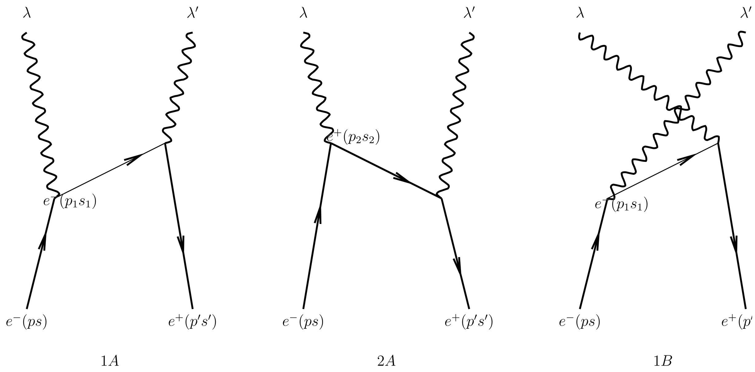
Feynman diagrams in noncovariant perturbation theory that contribute to the pair annihilation, e^-+e^+\to\gamma\gamma. — Figure 3:Feynman diagrams in noncovariant perturbation theory that contribute to the pair annihilation, $e^-+e^+\to\gamma\gamma$ .

Each row of Table 1 corresponds to a Feynman diagram that contributes to pair annihilation. The diagrams are shown in Figure 3. In diagrams $1A$ and $1B$ the intermediate state contains an electron; in $2A$ and $2B$ it contains a positron. The $A$ diagrams and the $B$ diagrams differ only in the order in which the two photons are emitted, that is, by a swap of photon labels $\lambda$ and $\lambda'$ .

Instead of wending our way through the combinatorics of creation and annihilation operators, we can directly write down the Feynman diagrams that contribute by combining the diagram fragments that appear in Figure 2 in such a way as to take us from the given initial state to the given final state. Once we have the diagram it is straightforward to write down the matrix elements, although we must be careful about normal ordering and sign changes.

Computing the Matrix Elements¶

Let us now compute the contribution of diagram $1A$ to the quantity $M$ , given in (80). From the diagram we see that the intermediate state contains the initial positron in mode $(p's')$ , the intermediate electron in mode $(p_1,s_1)$ , and the final photon in mode $\lambda$ . We write it as

\ket{k}=a^\dagger_\lambda b^\dagger_{p_1s_1} d^\dagger_{p's'}\ket{0},

(84)

and the sum on $k$ is interpreted as a sum on $(p_1,s_1)$ . We write $p_1=(E_1,\pvec_1)$ for the 4-momentum of the intermediate electrons, so that the energy denominator is

E_i-E_k= E-E_1-\omega.

(85)

The field part of the matrix element $\matrixelement{k}{H_T}{i}$ is obtained from Table 1 or from inspection of the Feynman diagram. It is

\matrixelement{k}{\mathcolon b^\dagger_{p_1s_1} a^\dagger_\lambda b_{ps}\mathcolon}{i} = \matrixelement{0}{d_{p's'}b_{p_1s_1}a_\lambda b^\dagger_{p_1s_1} a^\dagger_\lambda b_{ps} b^\dagger_{ps} d^\dagger_{p's'}}{0},

(86)

where in this case the normal ordering does nothing. Because the boson operators $a^\dagger_\lambda$ , $a_\lambda$ commute with all fermion operators, they can be migrated adjacent to the vacuum ket on the right, producing $a_\lambda a^\dagger_\lambda \ket{0}=\ket{0}$ . In what is left we have

\matrixelement{0}{d_{p's'}b_{p_1s_1} b^\dagger_{p_1s_1} b_{ps} b^\dagger_{ps} d^\dagger_{p's'}}{0} = \matrixelement{0}{b_{p_1s_1} b^\dagger_{p_1s_1} b_{ps} b^\dagger_{ps} d_{p's'}d^\dagger_{p's'}}{0},

(87)

where we have migrated $d_{p's'}$ four steps to the right, incurring four minus signs. But $d_{p's'}d^\dagger_{p's'}\ket{0}=\ket{0}$ , so what is left is

\matrixelement{0}{b_{p_1s_1} b^\dagger_{p_1s_1} b_{ps} b^\dagger_{ps}}{0}=1,

(88)

where we have used $b_{ps}b^\dagger_{ps}\ket{0}=\ket{0}$ and $b_{p_1s_1}b^\dagger_{p_1s_1}\ket{0}=\ket{0}$ , and finally $\braket{0}{0}=1$ .

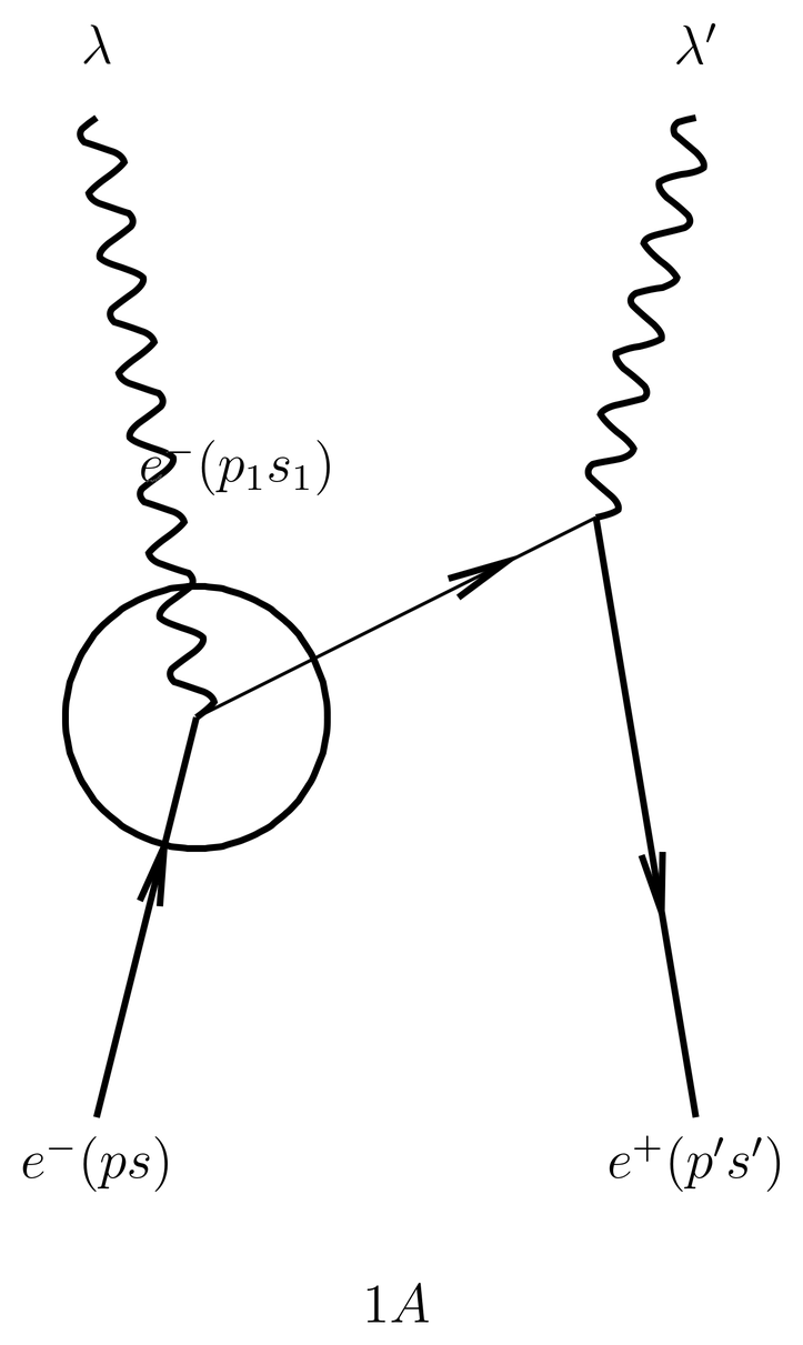
The matrix element \matrixelement{k}{H_T}{i} conserves 3-momentum at the first vertex (inside the circle), that is, the matrix element vanishes unless \pvec=\pvec_1+\kvec. — Figure 4:The matrix element $\matrixelement{k}{H_T}{i}$ conserves 3-momentum at the first vertex (inside the circle), that is, the matrix element vanishes unless $\pvec=\pvec_1+\kvec$ .

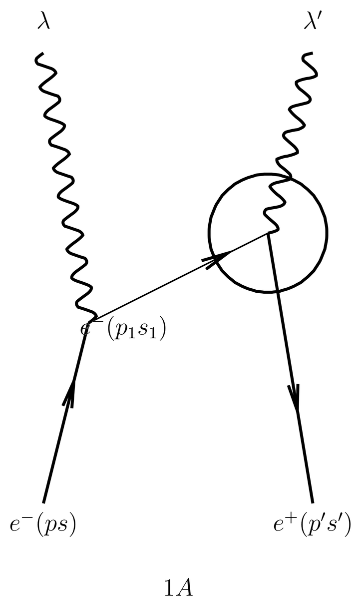
3-momentum is also conserved at the second vertex, that is, \matrixelement{n}{H_T}{k} vanishes unless \kvec'=\pvec'+\pvec_1. — Figure 5:3-momentum is also conserved at the second vertex, that is, $\matrixelement{n}{H_T}{k}$ vanishes unless $\kvec'=\pvec'+\pvec_1$ .

The rest of the matrix element is

\begin{aligned} \matrixelement{k}{H_T}{i}_{1A} &= {e\over V}\sqrt{{2\pi\over V}}\int d^3\xvec\, \sqrt{{m^2\over E_1E\omega}}\,(\ubar_{p_1s_1} \gammavec\cdot{\hat{\boldsymbol{\epsilon}}}^\cc u_{ps})\, e^{i\xvec\cdot(-\pvec_1-\kvec+\pvec)} \\ &= e\sqrt{{2\pi\over V}} \sqrt{{m^2\over E_1E\omega}}\, (\ubar_{p_1s_1}\gammavec\cdot{\hat{\boldsymbol{\epsilon}}}^\cc u_{ps}) \,\delta_{\pvec,\pvec_1+\kvec}, \\ \end{aligned}

(89)

where we have written simply ${\hat{\boldsymbol{\epsilon}}}$ for ${\hat{\boldsymbol{\epsilon}}}_\lambda$ . The Kronecker $\delta$ shows that momentum is conserved at the first vertex in diagram $1A$ , as shown in Figure 4.

It is convenient to promote the polarization 3-vector ${\hat{\boldsymbol{\epsilon}}}$ into a 4-vector by writing

\epsilon^\mu=(0,{\hat{\boldsymbol{\epsilon}}}),

(90)

which is similar to what we did with the electron spin when promoting the spin polarization 3-vector ${\hat{\mathbf{s}}}$ into the 4-vector $s^\mu$ . One difference is that the frame in which $s^\mu$ is purely space-like has an invariant meaning, that is, it is the rest frame of the electron. But the photon has no rest frame, so one can ask what the invariant meaning of (90) is. The answer is that it has no invariant meaning, rather Coulomb gauge is only valid in one frame, and that is the frame in which $\epsilon^\mu$ is purely space-like. In spite of this the definition is useful, as it allows us to write

\epsilonslash = \gamma^\mu \epsilon_\mu = -\gammavec\cdot{\hat{\boldsymbol{\epsilon}}},

(91)

so that

\matrixelement{k}{H_T}{i}_{1A}= -e\sqrt{{2\pi\over V}} \sqrt{{m^2\over E_1E\omega}}\, (\ubar_{p_1s_1}\epsilonslash^{\,\cc} u_{ps}) \,\delta_{\pvec,\pvec_1+\kvec},

(92)

where $\epsilonslash^{\,\cc}$ means $\gamma^\mu \epsilon^\cc_\mu$ .

We treat the matrix element $\matrixelement{n}{H_T}{k}$ similarly. The field part of the matrix element is

\matrixelement{0}{a_{\lambda'}a_\lambda\mathcolon d_{p's'}a^\dagger_{\lambda'}b_{p_1s_1}\mathcolon a^\dagger_\lambda b^\dagger_{p_1s_1} d^\dagger_{p's'}}{0}.

(93)

When we normal order and then migrate the boson operators to the right, we obtain $a_{\lambda'}a_\lambda a^\dagger_{\lambda'} a^\dagger_\lambda\ket{0}$ on the right, which reduces to simply $\ket{0}$ when we take account of the boson commutation relations and the fact that $\lambda\ne\lambda'$ . The latter fact follows from overall energy and momentum conservation, which will be discussed momentarily, which implies $\kvec'\ne\kvec$ . (This is easily seen in the center of mass frame, in which $\kvec=-\kvec'$ .) The remaining fermion operators can be reduced as before, showing that the field part of the matrix element (93) is just 1. Evaluating the rest of the matrix element as before, we obtain

\matrixelement{n}{H_T}{k}_{1A} = -e \sqrt{{2\pi\over V}} \sqrt{{m^2\over E'E_1\omega'}}\, (\vbar_{p's'}\epsilonslash^{\,\prime\cc}u_{p_1s_1}) \, \delta_{\kvec',\pvec'+\pvec_1}.

(94)

The final Kronecker- $\delta$ implies 3-momentum conservation at the second vertex of diagram $1A$ , as shown in Figure 5.

Putting the pieces from (80), (92), (94) and (85) together, we obtain the contribution of diagram $1A$ to the quantity $M$ ,

M_{1A} = e^2 {2\pi\over V} \sqrt{{m^2\over EE'\omega\omega'}} \,\sum_{p_1s_1} {m\over E_1} {(\vbar_{p's'}\epsilonslash^{\;\prime\cc} u_{p_1s_1})(\ubar_{p_1s_1}\epsilonslash^{\;\cc}u_{ps}) \over E-E_1-\omega}\,\delta_{\kvec',\pvec'+\pvec_1} \, \delta_{\pvec,\pvec_1+\kvec}.

(95)

The sum on $p_1$ really means a sum on the 3-momentum $\pvec_1$ , which can be done because of the Kronecker deltas. These force

\pvec_1=\pvec-\kvec=\kvec'-\pvec',

(96)

and they leave behind $\delta_{\pvec+\pvec',\kvec+\kvec'}$ which represents overall conservation of 3-momentum in the Feynman diagram. Although we continue to write $\pvec_1$ after the sum is carried out, it stands for the values in (96). Also, $E_1$ and $p_1$ are now understood to mean

E_1=\sqrt{m^2+|\pvec_1|^2},

(97)

and

p_1=(E_1,\pvec_1).

(98)

As for the spin sum over $s_1$ , it becomes a positive energy spin projector according to (39) and (153),

\sum_{s_1} u_{p_1s_1}\ubar_{p_1s_1} = {m+\pslash_1\over 2m} = \Pi_+(p_1).

(99)

Altogether, $M_{1A}$ is reduced to

M_{1A}= e^2 {2\pi\over V}\,\delta_{\pvec+\pvec',\kvec+\kvec'} \,\sqrt{{m^2\over EE'\omega\omega'}} {1\over 2E_1} {[\vbar_{p's'}\epsilonslash^{\;\prime\cc} (m+\pslash_1)\epsilonslash^{\;\cc}u_{ps}] \over E-E_1-\omega}.

(100)

The contribution of diagram $2A$ to the quantity $M$ can be computed in a similar manner. We summarize the results. The intermediate state is

\ket{k}=a^\dagger_{\lambda'}d^\dagger_{p_2s_2} b^\dagger_{ps}\ket{0},

(101)

the energy denominator is

E_i-E_k=E'-E_2-\omega',

(102)

the first matrix element (counting from the right) is

\matrixelement{k}{H_T}{i}_{2A} = -e\sqrt{{2\pi\over V}} \sqrt{{m^2\over E'\omega'E_2}}\, (\vbar_{p's'}\epsilonslash^{\;\prime\cc}v_{p_2s_2}) \,\delta_{\pvec',\kvec'+\pvec_2},

(103)

where the minus sign comes from normal ordering and fermion anticommutators, and the second matrix element is

\matrixelement{n}{H_T}{k}_{2A}= e\sqrt{{2\pi\over V}} \sqrt{{m^2\over E\omega E_2}}\, (\vbar_{p_2s_2}\epsilonslash^{\;\cc}u_{ps})\, \delta_{\kvec,\pvec_2+\pvec}.

(104)

Now when we do the $p_2$ sum we get

\pvec_2=\kvec-\pvec=\pvec'-\kvec',

(105)

and afterwards we understand $\pvec_2$ to stand for one of these values. We also understand that

E_2=\sqrt{m^2+|\pvec_2|^2},

(106)

and

p_2=(E_2,\pvec_2).

(107)

We also get a Kronecker delta representing overall momentum conservation. As for the $s_2$ sum, it can be expressed in terms of the negative energy projector, again via (39) and (153),

\sum_{s_2}v_{p_2s_2}\vbar_{p_2s_2}= {\pslash_2-m\over 2m} = -\Pi_-(p_2).

(108)

Altogether, this gives

M_{2A}= -e^2 {2\pi\over V}\,\delta_{\pvec+\pvec',\kvec+\kvec'} \,\sqrt{{m^2\over EE'\omega\omega'}} {1\over 2E_2} {[\vbar_{p's'}\epsilonslash^{\;\prime\cc} (\pslash_2-m)\epsilonslash^{\;\cc}u_{ps}] \over E'-E_2-\omega'}.

(109)

The amplitudes $M_{1B}$ and $M_{2B}$ are obtained from $M_{1A}$ and $M_{2A}$ , (100) and (109), by swapping $\lambda\leftrightarrow\lambda'$ , that is, $\kvec\leftrightarrow\kvec'$ , $\omega\leftrightarrow\omega'$ and $\epsilonslash^{\;\cc}\leftrightarrow\epsilonslash^{\;\prime\cc}$ .

The conservation of 3-momentum at the vertices of the Feynman diagrams means that the 3-momentum of the intermediate state is equal to the 3-momentum of both the initial and final states. And the energies of the initial and final states are forced to be equal by the energy-conserving delta-function in the transition probability (79), in the limit $t\to\infty$ . But the energy of the intermediate state is not equal to the energies of the initial and final states. If it were, the energy denominators $E_i-E_k$ , which appear in (85) and (102), would vanish. The intermediate states arose originally in the Dyson series from a resolution of the identity, which means a sum over all states, regardless of energy.

The Feynman Propagator¶

The amplitudes $M_{1A}$ and $M_{2A}$ can be combined. These amplitudes have many factors in common, so computing the sum boils down to adding the parts that are different, that is, combining the fractions

{1\over 2E_1} {m+\pslash_1 \over E-E_1-\omega}- {1\over 2E_2} {\pslash_2-m \over E'-E_2-\omega'}.

(110)

The algebra of doing this is straightforward. What is interesting is that the result can be written in covariant form.

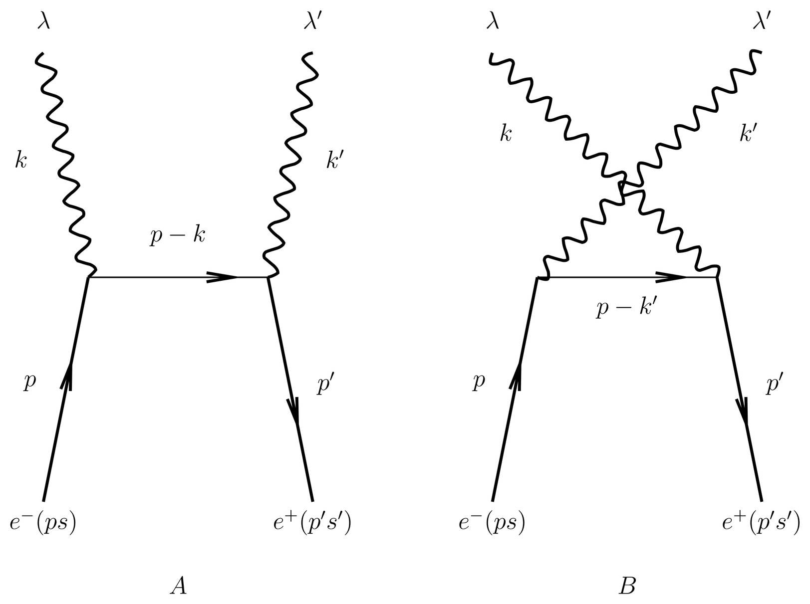
Feynman diagrams A and B that appear in covariant perturbation theory. All lines are labelled by their 4-momenta, and 4-momentum is conserved at each vertex. But the 4-momentum of the internal or virtual electron-positron line is not “on mass shell.” — Figure 6:Feynman diagrams $A$ and $B$ that appear in covariant perturbation theory. All lines are labelled by their 4-momenta, and 4-momentum is conserved at each vertex. But the 4-momentum of the internal or virtual electron-positron line is not “on mass shell.”

We are using noncovariant or “old-fashioned” perturbation theory. It is based on Hamiltonians and the selection of a privileged Lorentz frame. The use of a Hamiltonian, which is the generator of time translations, always implies a privileged Lorentz frame, since the time of one Lorentz frame is not the same as the time of another. Thus, Hamiltonian methods are never covariant (at least this is the usual point of view). Noncovariant perturbation theory is not wrong, but it is not as efficient or as elegant as covariant perturbation theory. In covariant perturbation theory, diagrams $1A$ and $2A$ combine into a single diagram $A$ , and likewise diagrams $1B$ and $2B$ combine to a single diagram $B$ . These diagrams are illustrated in Figure 6.

To combine the fractions (110) we first use (96) and (105) to express $p_2$ in terms of $p_1$ ,

p_2=(E_2,\pvec_2) = (E_1,-\pvec_1).

(111)

We then use overall energy conservation, $E+E'=\omega+\omega'$ , to express the second denominator in (110) as

E'-E_2-\omega' = -(E-\omega+E_1).

(112)

These allow us to write the expression (110) as

{1\over 2E_1} \Bigl( {\pslash_1+m \over E-\omega-E_1} + {\pslash_2-m \over E-\omega+E_1}\Bigr) = {1\over 2E_1} {(E-\omega)(\pslash_1+\pslash_2) + E_1(\pslash_1-\pslash_2+2m) \over (E-\omega)^2 - E_1^2}.

(113)

But $\pslash_1+\pslash_2=2E_1\gamma^0$ and $\pslash_1-\pslash_2=-2\pvec_1\cdot\gammavec$ , so the fractions combine to

{(E-\omega)\gamma^0 - (\pvec-\kvec)\cdot\gammavec +m\over (E-\omega)^2 - (\pvec-\kvec)^2 - m^2} = {\pslash-\kslash+m\over (p-k)^2-m^2} = D_F(p-k),

(114)

where we define the photon 4-momentum $k=(\omega,\kvec)$ , where dot products are understood in the 4-dimensional sense, for example, $(p-k)^2 = (p^\mu-k^\mu)(p_\mu-k_\mu)$ , and where for any $p$ ,

D_F(p) = {\pslash+m\over p^2-m^2}.

(115)

The function $D_F$ is called the Feynman propagator; it is a kind of Green’s function for the free particle Dirac equation.

We can now write out the sum of amplitudes,

M_A=M_{1A}+M_{2A} = e^2 {2\pi\over V}\,\delta_{\pvec+\pvec',\kvec+\kvec'} \,\sqrt{{m^2\over EE'\omega\omega'}}\, [\vbar_{p's'}\epsilonslash^{\;\prime\cc} D_F(p-k)\epsilonslash^{\;\cc}u_{ps}],

(116)

which is the amplitude associated with diagram $A$ in Figure 6. We obtain the amplitude for diagram $B$ by swapping photon labels,

M_B =e^2 {2\pi\over V}\,\delta_{\pvec+\pvec',\kvec+\kvec'} \,\sqrt{{m^2\over EE'\omega\omega'}}\, [\vbar_{p's'}\epsilonslash^{\;\cc} D_F(p-k')\epsilonslash^{\;\prime\cc}u_{ps}].

(117)

To complete the calculation of the cross we must average over initial electron and positron states (if we are thinking of unpolarized beams). This process is rather tedious so we will stop here.

Courses on quantum field theory normally begin with covariant quantization and perturbation theory, but without any of the background given in these notes which show how those topics are connected with the rest of quantum mechanics or how they developed historically.

Perhaps the biggest question left unanswered by these notes is why the first quantized Dirac equation gives such good results, if we ignore the negative energy solutions. We have explained that the first quantized theory, prior to the introduction of hole theory, is physically incomplete, becuase of a lack of interpretation of the negative energy solutions. And we have indicated how those interpretational problems are solved by the introduction of field theory. But from a logical standpoint it would be nice to show how and in what sense the first quantized theory is an approximation to field theory. That is an interesting subject that is not usually covered in courses in quantum field theory, which mostly deal with problems that can be solved by the Born approximation. It is perhaps a question that will be covered in a future set of notes.

Problems¶

Problem 1.

The purpose of this problem is to derive the equations of motion (\eqr\cn.50) from the Lagrangian (\eqr\cn.57), for which the independent fields are $\psi$ , $\psibar$ and $\Avec$ , the last of which is understood to be transverse. The work is carried out in Coulomb gauge.

It is best not to use the Euler-Lagrange equations (12), but rather to vary the action $S=\int L\,dt$ with respect to the independent fields, and to demand that $\delta S=0$ for all such variations. For practice on this you may see how we obtained Maxwell’s equations in The Electromagnetic Lagrangian. Note that when we vary $\psi$ or $\psibar$ , there is a nonvanishing variation $\delta\rho$ , because of (57), which causes a nonvanishing variation $\delta\Phi$ , because of (56). If we write $S_\text{Coul}$ for the Coulomb contribution to the action,

S_\text{Coul}=\int dt\, {1\over2}\int d^3\xvec \, \rho\Phi,

(118)

show that under variations of $\psi$ or $\psibar$ we have

\delta S_\text{Coul} = \int dt \int d^3\xvec\, \delta\rho\,\Phi.

(119)

Then use this to derive the covariant Dirac equation (54), driven by the electromagnetic field.

To derive Maxwell’s equations driven by the Dirac field, (55), we must vary with respect to $\Avec$ . Note that if $\Vvec$ is any vector field and if we demand that

\int d^3\xvec\, \Vvec(\xvec)\cdot\delta\Avec(\xvec)=0

(120)

for all transverse variations $\delta\Avec$ , then we cannot conclude that $\Vvec(\xvec)=0$ , only that $\Vvec_\perp(\xvec)=0$ . That is because

\int d^3\xvec\, \Vvec\cdot\delta\Avec = \int d^3\xvec\, (\Vvec_\parallel+\Vvec_\perp)\cdot\delta\Avec =\int d^3\xvec\, \Vvec_\perp\cdot\delta\Avec,

(121)

where we use (31). Therefore when you vary $\Avec$ you will obtain a transverse equation of motion. Show that the longitudinal component of this equation is implied by Coulomb gauge, so that overall the equation of motion is equivalent to Maxwell’s equations driven by the Dirac current, (55).

This calculation is an example of how Coulomb gauge takes us through noncovariant intermediate steps but produces covariant results. It also shows that the Lagrangian (62) gives the correct equations of motion (for the model we are using).

Problem 2.

Positrons were first observed by Anderson in 1932 in cosmic ray tracks in a cloud chamber. The experimental apparatus consisted of a series of parallel plates of lead (a high $Z$ material), separated by air gaps. Cosmic rays at the earth’s surface are mainly muons, some of which have very high energies. In the Anderson apparatus, a high energy muon, passing close to a nucleus of lead and being accelerated in the electric field, produced a gamma ray. This process is called {\it Bremsstrahlung} (German for ``braking radiation’'). The gamma ray, in turn, passing near a lead nucleus in one of the lower plates, produced an electron-positron pair.

To model this process, we add a term to the perturbing Hamiltonian $H_1=H_\text{Coul}*+H_T$ , given by (74), to account for the interaction with the nucleus,

H_ext = \int d^3\xvec\, \mathcolon\rho(\xvec)\Phi_ext(\xvec)\mathcolon = -e \int d^3\xvec \mathcolon\psibar(\xvec)\gamma^0 \Phi_ext(\xvec)\psi(\xvec):.

(122)

This is exactly how we treated the field of the nucleus Mott scattering (see (12) and Scattering by an External Potential $\Phi(\xvec)$ ). In effect, we are dividing the electromagnetic field into a $c$ -number field (from the nucleus) plus the quantized field. If we wish to model the lead nucleus as a point charge, we can take $\Phi_ext(\xvec)= Ze/r$ , but for this problem we will leave $\Phi_ext$ unspecified. Thus, the perturbing Hamiltonian is now

H_1=H_\text{Coul} + H_T + H_\text{ext}.

(123)

(a) Consider a process in which a photon passes close to a nucleus, and an electron-positron pair is produced. (This process cannot happen in free space because of energy-momentum conservation.) Let $(ps)$ be the 4-momentum and spin of the outgoing electron, let $(p's')$ be the 4-momentum and spin of the outgoing positron, let $\lambda = (\kvec,\epsilonvec)$ be the mode of the incident photon. Also write

\begin{aligned} p^\mu & = (E,\pvec), \end{aligned}

(124)

\begin{aligned} p^{\prime\mu} &= (E',\pvec'), \end{aligned}

(125)

\begin{aligned} k^\mu &= (\omega,\kvec). \end{aligned}

(126)

Find and draw all Feynman diagrams which contribute to this process at lowest order in $\alpha =e^2$ . Count the external potential $\Phi$ as containing one power of $e$ (since we are thinking of $\Phi=Ze/r$ ). Indicate the interaction with the nucleus by an $\times$ drawn next to an electron or positron line, as in Figure 1.

(b) Write the transition probability as in (79), which defines $M$ . Pick out two Feynman diagrams which differ from one another only in the time ordering of the creation of the outgoing electron and positron. Work out in detail the contribution to $M$ from each of these Feynman diagrams. Express your answer in terms of the Fourier transform of the potential $\tilde\Phi(\qvec)$ , as we did with Mott scattering.

(c) Combine the two terms, and express the result in terms of the Feynman electron propagator (115).

The steps remaining to convert $M$ into a cross are straightforward but tedious so we will stop at this point.

52. Electromagnetic Interactions With the Dirac Field

Introduction¶

The Dirac Field Interacting With an External Electromagnetic Field¶

Scattering by an External Potential Φ(x)\Phi(\xvec)Φ(x)¶

Summing and Averaging over Spin States¶

Traces of Products of γ\gammaγ-Matrices¶

The Mott Cross Section¶

Covariant Lagrangian for the Interacting Dirac and Electromagnetic Fields¶

Coulomb Gauge and Covariant Quantization¶

Coulomb Gauge in the “Classical” Theory¶

The Quantum System¶

Electron-Positron Annihilation¶

Computing the Matrix Elements¶

The Feynman Propagator¶

Problems¶

Scattering by an External Potential $\Phi(\xvec)$ ¶

Traces of Products of $\gamma$ -Matrices¶