43. Scattering of Radiation by Matter
Introduction
In the previous set of notes we treated the emission and absorption of radiation by matter. In these notes we turn to the scattering of radiation by matter. As before, the material system in question can be almost anything (atom, molecule, nucleus, etc), but when it is necessary to be specific we shall for simplicity assume that it is a single-electron atom. The formalism is easily extended to other types of material systems.
We shall see that in a certain sense the emission and absorption of radiation are special cases of the scattering of radiation, in which the frequency of the initial photon is close to a resonance frequency of the material system (the Einstein frequency connecting two energy eigenstates). In such cases it is partly a matter of preference how one should view the process, but in some respects the scattering point of view is more fundamental and elegant.
Applications
The applications of the theory developed in these notes are very broad. Almost any situation in which radiation passes through a gas affords an example of the physics we shall describe here. For example, in infrared and Raman scattering experiments radiation is passed through a molecular gas and the absorption spectrum or scattering cross is measured, providing a primary source of information about the structure of molecules.
Another example involves radiation passing through the Earth’s atmosphere. The atmosphere is mostly transparent to sunlight, but there is some scattering, especially at the higher (blue) frequencies. This is Rayleigh scattering, which is discussed in 12. The higher frequencies are more strongly scattered because they are closer to certain resonances in the ultraviolet. As we shall see, the cross for scattering rises rapidly as a function of frequency as we approach a resonance. This is the reason the sky is blue: When we look at a part of the sky away from the sun, the blue light we see is sunlight scattered by the air along our line of sight.
The Earth in turn radiates thermal radiation in the infrared that must pass through the atmosphere to reach outer space where it escapes. This radiation has a frequency range that covers the vibrational transitions of most simple molecules, so it is strongly scattered by several types of molecules such as the greenhouse gases , and . Thus an infrared photon leaving the Earth’s surface must diffuse through the atmosphere in a random walk, a process that is much slower than passing straight through. The greenhouse gases act like a blanket, keeping the Earth warm. Notice that the atmosphere makes it easy for radiation to get in at optical frequencies, and difficult to get back out at infrared frequencies.
There are many examples in astrophysics where the scattering or absorption of radiation by matter is important. For example, sunlight passing through the cooler outer layers of the sun’s atmosphere produces an absorption spectrum (the dark Fraunhoffer lines) that give information about the chemical species occurring in the sun and the physical conditions in its atmosphere. Similar information is available for other stars. For another example, transport of energy by radiation is important in the interior of stars, in which photons undergo repeated scattering by free electrons in the plasma and by bound electrons in atoms (if the atoms are not completely stripped, it depends on circumstances) and slowly diffuse upward toward the surface. In many stars such as the sun this radiative transport dominates the energy transport at certain radii, while at other radii convective transport is dominant.
The interaction of photons with matter is also important in nuclear physics. In the M"ossbauer effect, for example, gamma ray photons emitted in the decay of a nucleus are used to excite other nuclei, lifting them from their ground state into an excited state. See The Nucleus and the M"ossbauer Effect. The resonance is very narrow, however, and the photon can be shifted out of resonance by a Doppler shift involving only small velocities. The M"ossbauer effect provided the first clear experimental demonstration of the red shift that photons suffer on climbing out of a gravitational field. This effect implies that clocks run at different rates in different regions of a gravitational field. It is one of the conceptual corner stones of general relativity.
The Scattering Problem
We shall consider the reaction
in which an atom in state interacts with an incident photon , which leaves the atom in state and produces the scattered photon . We will write , for the modes of the incident and scattered photons, where is a polarization index, as described in The Mode Expansion. We will assume that , since otherwise there is no scattering. If , the scattering is elastic (the initial and final atomic states are the same), and by conservation of energy we have , where and are the frequencies of the photons with modes and . If , the scattering is inelastic, and we have . In this case the final atomic state may either be higher or lower in energy than the initial state , depending on circumstances. We will use box normalization in our analysis, so the indices , , etc are discrete. With a few changes, the states and can be interpreted as belonging to a molecule, nucleus, or other material system, rather than an atom.
We shall treat the scattering reaction (1) by means of time-dependent perturbation theory, developed in 34. Time-Dependent Perturbation Theory. As we shall see, we will have to make some extensions of that theory for the application at hand. Our earlier presentation of time-dependent perturbation theory was stated in a general notation, in which is an initial state, is a variable final state that we must sum over to get useful transition probabilities, and is an intermediate state. These initial, final and intermediate states will be identified with particular states in our atom-field system, so we will switch back and forth between the general notation and the one specific to our problem.
Specifically, we have one photon in both our initial and final states. We will write these states in a variety of ways,
The energies of these states are
where and are the energies of the two atomic states. The Einstein frequency connecting the initial and final states is
where .
The problem will be to compute the differential cross , where refers to the direction of the outgoing photon (in mode ). The differential cross is a function of the mode of the initial photon , the two atomic states and , and of the polarization and direction of the final photon, whose mode is . The energy of the final photon is determined by conservation of energy.
The Transition Amplitude Vanishes at First Order in 
We will take the Hamiltonian for the interaction of the matter with the radiation to be , where
We write our Hamiltonian as so as not to confuse it with the Hamiltonian that is used in the general theory of time-dependent perturbation theory. We will have to identify with for our particular problem, and with . Although we have written as a single-electron system, very little of the following analysis depends on this and our results, as mentioned, will be valid also for molecules, nuclei, and other systems.
The Hamiltonian is ordered in powers of the vector potential , which represents physically the amplitude of the light wave. That is, is , is , including the term since , and is .
The transition amplitude in first order time-dependent perturbation theory is given by (40), which we reproduce here:
For our application we must replace by , but if we only wish to work to first order in we can ignore compared to . Thus we make the replacement,
in (8). The fields and have Fourier series (22) and (24) in terms of the modes of the field. If we write out these series, suppressing all factors except the creation and annihilation operators, then they have the structure,
where we are careful to use the index as a dummy variable of summation, so as not to confuse it with the indices and of the incident and scattered photons.
Now focusing on the field part of the matrix element (9), we see that the annihilation operator does not contribute to the transition amplitude, because it acts on a state with a single photon, , and either produces a state with zero photons (if ) or annihilates it (if . In either case, the resulting state is orthogonal to the state , and gives zero when the scalar product is taken. Similarly, the creation operator in the Fourier series (10) acts on the single photon state and produces a two-photon state, which is necessarily orthogonal to any one-photon state such as . Again, the field part of the scalar product vanishes. Thus we find
and there is no contribution to the scattering amplitude at first order in .
More generally, in any vacuum expectation value of a product of creation and annihilation operators, something like
the answer vanishes unless the number of ’s and the number of ’s are equal. In particular, the answer vanishes if the total number of ’s and ’s is odd.
We see that for our problem, we must go to second order in to find a nonvanishing contribution; this will involve second order perturbation theory.
Second-Order Time-Dependent Perturbation Theory
This is the first time we have had an application of second-order time-dependent perturbation theory, so we shall return to the formalism of 34. Time-Dependent Perturbation Theory\ and develop the theory at second order, using the notation of those notes. In particular, the Hamiltonian is . The second-order contribution to the transition amplitude in the interaction picture is given by (38) in the general case in which in the Schr"odinger picture is allowed to depend on time. For our scattering application, is time-independent, so we can do the time integrations appearing in (33). The integral in the first order term in (33) was done already in The Case that is Time-independent, with the result shown in (40) and reproduced above in (8). As for the integrals in the second order term in (34), we first do the integration, finding,
Recall that the sum on is a sum over “intermediate states” that came from the insertion of a resolution of the identity between the two Hamiltonian factors in (34). We combine the phase factors in (13), using the identity,
and then we do the integration,
Of the two major time-dependent factors in the square brackets in (16), the first one,
is the same time-dependent factor that appears in the first order term shown in (8). Notice that this factor is independent of and can be taken out of the sum in (16). When squared to produce a probability, this factor produces a quantity proportional to time multiplied times a function of frequency that gets narrower as time gets longer,
where
See (51) and (52). The fact that the result is proportional to time is essential for getting a transition rate (a probability per unit time), and the emerging -function in the limit is necessary for energy conservation, as explained in 34. Time-Dependent Perturbation Theory. In fact, as explained in Short-Time Behavior, we do not really have to take to , it need only be long enough for certain initial transients to die away. These transients are related to the artificiality of the initial conditions, and are nonphysical.
The initial conditions for the scattering problem considered in these notes contain an artificial element, as did the initial conditions in the potential scattering problem considered in Application: Potential Scattering. That is, we are assuming that at the atom is known to be in the state and the field consists of a single photon in mode . This mode is a plane wave that fills up all of space, including the region occupied by the atom. It would be impossible to set up such initial conditions experimentally, since there is no way for a light wave to get into the region occupied by the atom without interacting with it. A more realistic set of initial conditions would be a wave packet made up out of single photon states that initially is remote from the atom and not interacting with it. To treat such wave packets, however, would require a more sophisticated formalism than we are using here, so we will stick with the initial conditions we have chosen. The price we pay, however, is the appearance of initial transients without physical significance.
The second major time-dependent term inside the square brackets in (16) is just such a transient. This term, when squared, does not produce something proportional to time, but rather just gives bounded oscillations that go to zero in the limit after we divide by time. Thus, they do not contribute to the transition rate. This is because the frequency occurring in that term is not independent of . The same is true for the cross terms that arise when the sum of the two major time-dependent terms in (16) is squared. Thus, if all we are interested in is the transition rate and not the initial transients, we can drop the second major time-dependent term in (16).
The result is an effective transition amplitude at second order that is proportional to the time-dependent factor (17), the same factor that occurs at first order. Combining the first and second order terms, we obtain an effective transition amplitude,
where we have taken the denominator appearing in (16) and written it as . The result is the “energy denominator” seen in the second order contribution in (20). Recall that we had such energy denominators also in second-order bound state perturbation theory (see 23. Bound-State Perturbation Theory). We drop the zeroth order contribution to the transition amplitude since for our scattering problem (since ).
The Photon Scattering Amplitude at Order 
For our application in (20) must be replaced by . At first order of perturbation theory, this gives the matrix element
As we have just seen, however, the contribution to this matrix element from vanishes. But at second order in we must keep the term . This is the second-order Hamiltonian taken in first-order perturbation theory. Likewise, in the second order term of the general expression (20), we can simply replace by , ignoring , if we wish to work to second order in . That is, we take the first-order Hamiltonian at second order perturbation theory. Altogether, the effective transition amplitude for our scattering problem, valid through order , is
where and are given by (5) and states and are given by (2).
in First-Order Perturbation Theory
We begin with the term
Squaring the Fourier series (22) for , we obtain a product series with the structure,
where we suppress all factors except the creation and annihilation operators. This allows us to concentrate on the photon part of the matrix element (23). We see that there are four types of products of creation and annihilation operators that occur in . The product of the two annihilation operators does not contribute to the transition amplitude, since it acts on the single photon state producing zero. Likewise, the product of the two creation operators does not contribute, since it acts on creating a three-photon state that is orthogonal to the one-photon state . The product of the annihilation operator times the creation operator, , does contribute, however, as long as and . That is, the photon destroyed by must be the incident photon, and the one created by must be the scattered photon. Taking into account the other factors in the Fourier series, this product of operators corresponds to the product of polarization vectors and the product of phase factors . Similarly, the product of the creation operator times the annihilation operator contributes as long at and , and in this case the product of polarization vectors is and the product of phase factors is . The terms that contribute are those that have a total of two annihilation and two creation operators between the vacuum bra and vacuum ket.
Thus out of the double infinite series (24) for , only two terms contribute to the transition amplitude, and both have the same product of polarization vectors and the same phase factors. The contributions of these two terms are equal. It is now easy to do the photon part of the matrix element, leaving only an atomic matrix element. The result is
where the leading factor of 2 comes from the fact that we have two identical terms, and where we have made the abbreviations, , .
In the following we shall use the dipole approximation, in which . As explained in 42. Emission and Absorption of Radiation, this approximation is equivalent to , where is the size of the atom and is the wave length of the radiation. This is an excellent approximation for atoms at optical frequencies, where the ratio is less than 10-3. This causes the atomic matrix element in (25) to become simply . We see that the -term only contributes to elastic scattering. Altogether, the matrix element becomes
Feynman Diagrams
Before proceeding to the term, we show how the terms of the perturbation series are associated with Feynman diagrams. A Feynman diagram is basically a space-time diagram showing the interactions of the particles. The diagrams correspond to terms in the transition amplitude; thus, each diagram is a complex number.
The time sequence of particle interaction in a Feynman diagram comes from the Dyson series in time-dependent perturbation theory. The Dyson series is given by (27), reproduced here:
This is a power series in , a solution of the time-dependent Schr"odinger equation in the interaction picture with initial condition . The Hamiltonian is in the interaction picture; it is time-dependent even when (in the Schr"odinger picture) is not, hence at different times do not commute.
We will use the second order term of the Dyson series to illustrate the time ordering. In this term the various times satisfy
where the initial time is 0, and are a pair of sequenced intermediate times, and is the final time. This leads to a language for describing the second order term of the Dyson series: we say that the initial state is unchanged until time when it is acted upon by , after which it is unchanged until time when it is acted upon by , after which it is unchanged until the final time . The second order contribution to the transition amplitude is the sum (that is, the integral) of all such contributions, for all possible (ordered) values of and .
Similarly, the first order term involves interacting with at one intermediate time , and the zeroth order term involves no interaction. The pattern is clear for terms of any order.
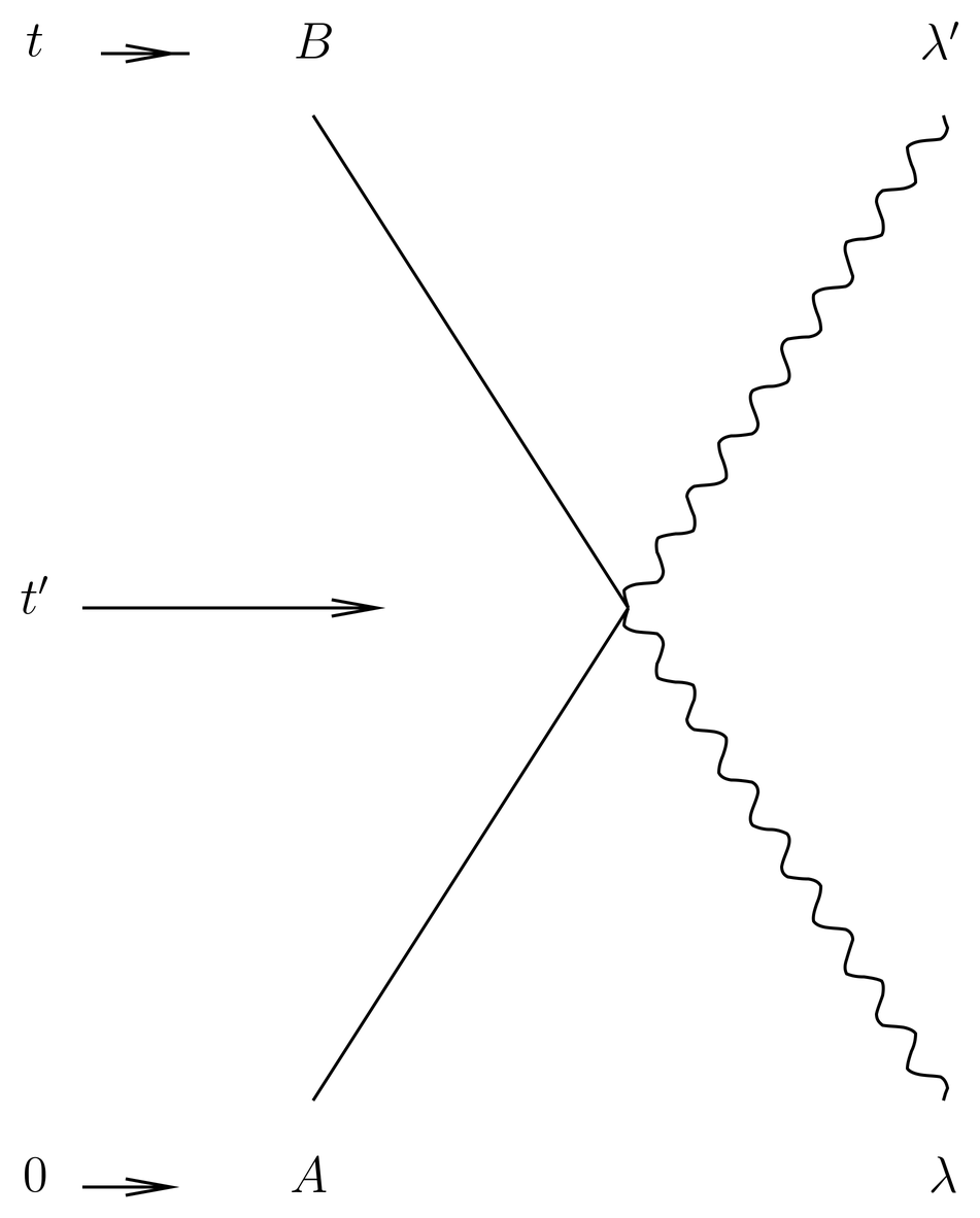
Figure 1:The seagull diagram. The four-point vertex describes the action of at intermediate time , which annihilates the incident photon in mode , creates the scattered photon in mode , and connects initial atomic state with final state . Time runs from bottom to top in the diagram, with the time sequence .
To return to our problem, the term involves the second order Hamiltonian, but comes from the first order term in the Dyson series. Thus there is one interaction with at one intermediate time. This interaction destroys the incident photon and creates the final photon , and connects the initial atomic state with the final atomic state . The Feynman diagram is shown in Figure 1; it is called a “seagull” diagram. In the diagram time increases from bottom to top. The atom lines are straight lines, and the photon lines are curvy. The single interaction with is an example of a 4-point vertex, that is, an interof four lines. Four-point vertices are created by the term in the Hamiltonian, because of the structure of the product of the two Fourier series discussed above.
The term in Second Order Perturbation Theory
Now we turn to the second order term in the transition amplitude, extracted from (22):
where we use the general notation for the initial state , the final state , and the intermediate state . In our problem runs over a complete set of state of the matter plus field system, and in particular, it must include states of any number of photons. But and contain only one photon, and can create or destroy only one photon, so the only intermediate states that give nonvanishing matrix elements are those with either zero or two photons. Thus there are two cases.
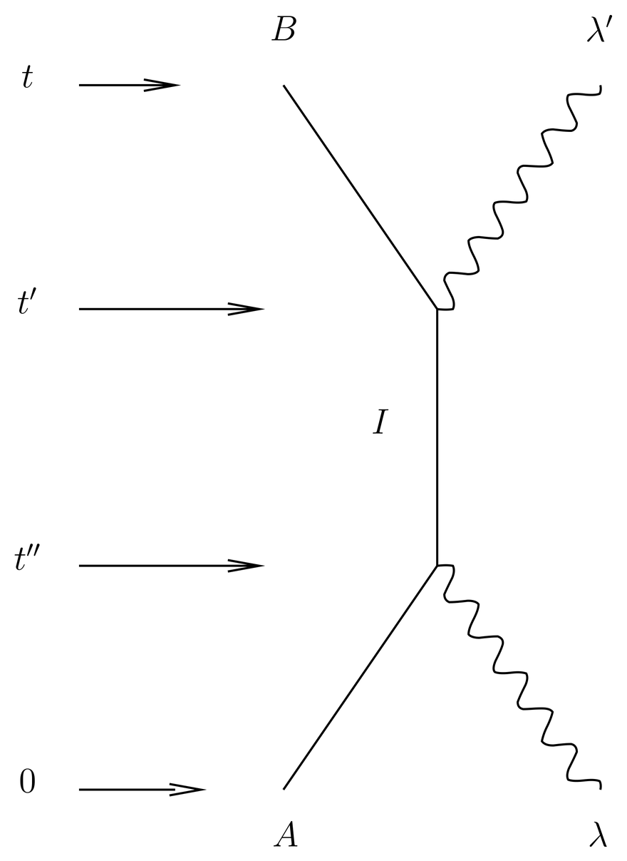
Figure 2:In case I, the incident photon is destroyed before the final photon is created. There are zero photons in the intermediate state.
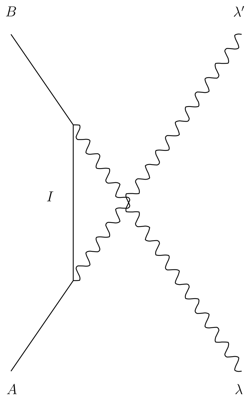
Figure 3:In case II, the final photon is created before the incident photon is destroyed. There are two photons in the intermediate state.
In case I, the intermediate state contains zero photons. The first application of (at the first intermediate time, in our notation) annihilates the incident photon , and the second application of (at the second intermediate time, in our notation) creates the final photon . In case II, the intermediate state contains two photons, which must be in modes and . The first application of creates the final photon and the second (later) application of destroys the incident photon . Thus we have
where refers to an intermediate atomic state. The Feynman diagrams for cases I and II are given in Figs.~Figure 2 and Figure 3.
We may now evaluate the contributions of cases~I and II to the sum (29). The initial and final energies and , in the general notation, are translated into the notation of this problem by (3). In case~I, the energy of the intermediate state, in the general notation, becomes , the energy of the intermediate atomic state, in the notation of this problem. Thus, in case~I, the energy denominator in the sum (29) becomes
where . Also, the second matrix element in (29) is interpreted as
after using (6) for and evaluating the field part of the matrix elements. We have dropped the term involving , since it is of order compared to the term (this is equivalent to the dipole approximation, in which we set ). What is left is a purely atomic matrix element. Similarly, the first matrix element in (29) is interpreted as
Altogether, the contribution of case~I, that is, the Feynman diagram in Figure 2, to the sum (29) is
Similarly, we find the contribution of case~II, that is, the Feynman diagram in Figure 3. It works out to be
Putting the pieces together, the total transition amplitude (22) becomes
where is an abbreviation,
Note that is dimensionless. Note also that the sum over intermediate atomic states must include states of the continuum; for these, the notation is an abbreviation for an integral over the continuous quantum numbers, as well as a sum over the discrete ones.
The Kramers-Heisenberg Formula
Let us fix the mode of the incident photon, the initial and final atomic states and , and the polarization of the outgoing photon. Then the final state is , in which only the final wave vector of the outgoing photon is variable. We must sum the transition probabilities over a collection of final states to obtain the differential cross , exactly as we did in the simpler scattering problems considered in 34. Time-Dependent Perturbation Theory.
Let be a chosen direction for the outgoing photon, and let us construct a small cone of solid angle about this direction, as in Fig.~\figr\tdpt.5. The prime on means that it is a solid angle referring to the outgoing photon. Let us also define as the magnitude of as determined by conservation of energy, that is,
which follows from [see (4)].
The differential cross , for fixed values of , , and , is the transition probability per unit time per unit solid angle of the outgoing photon per unit incident flux of the incoming photon for transitions in which lies in the small cone just described, in the limit that time is long enough for the initial transients to die away. We also take to get rid of the box and to obtain physical results. That is, we can write
As we have done in 34. Time-Dependent Perturbation Theory, we sum over all wave vectors in the small cone, and do not try to enforce energy conservation by hand. Taking the factors in (39) one at a time, the incident flux of photons is , since there is one incident photon in the box travelling at the speed of light. The sum over final photon states becomes an integral in the limit ,
Finally, the square of the transition amplitude (36) becomes
where we have used (51). The matrix element depends on because it contains the polarization vectors . The direction of is determined by the cone, that is, the choice of .
Putting the pieces together, we find
or, upon doing the integral,
where
and where in the final expression it is understood that , since the direction of is fixed by the small cone and the magnitude by the energy-conserving -function. Also, is determined by energy conservation. (43), with given by (37), is the Kramers-Heisenberg formula. It was first derived by methods of the old quantum theory, and is important historically because the calculation led Heisenberg to realize that a fundamental difference between classical mechanics and quantum mechanics is that in quantum mechanics classical observables are replaced by noncommuting operators. (Heisenberg thought of these operators as matrices, hence the name “matrix mechanics” for the first version of quantum mechanics).
The quantity is called the classical radius of the electron. It is called “classical” because the expression does not involve and because it has a classical interpretation: it is the radius outside of which the integrated energy in the electric field of the electron, , is equal to the rest-mass-energy of the electron (apart from constants of order unity). At one point physicists were playing with the idea that the observed mass of the electron might be purely energy in the field. This idea was not very successful, however, and later developments in quantum electrodynamics showed that it was rather naive. However, the general idea points to a paradox of classical electromagnetism, namely, the total integrated energy of the electric field of a point particle, if it is carried all the way to and if Coulomb’s law is valid all the way to , is infinite. As we shall see when we study the Lamb shift, the quantum theory also leads (nominally) to an infinite mass of the electron. In addition to the infinite zero-point energy, it is one of the infinities that appear in quantum field theory.
In any case, the cross-(43) is proportional to
where is the Bohr-radius. Since this is a very small area by atomic standards. The geometrical cross of the atom is roughly , and this is roughly the cross for the scattering of electrons of several eV of energy by an atom. But quantity , which sets the scale for photon scattering, is much smaller.
Can the dimensionless quantity enhance the cross for photon scattering? One can see from the definition (37) that all quantities appearing there are of order unity in atomic units, if the states and have reasonably small quantum numbers. If, however, one of the denominators should be small, then can be large and lead to an enhancement. In fact, the denominator in the first term in (37) is small if , that is, if the incident photon has the right energy to raise the atom from its initial state to an intermediate state . This intermediate state must be higher in energy, since . If this is the case, the incident photon is in resonance with one of the excitation frequencies of the atom. Similar interpretations can be given to the second term, although in that term the outgoing photon is emitted before the incident photon is absorbed, as indicated by the Feynman diagram in Figure 3.
If is chosen so that there are no resonances (none of the denominators in (37) is small) then the cross-for atom-photon scattering is comparable to , and is very small by atomic standards. This is why ordinary gases are transparent to radiation at optical frequencies, unless very thick.
We will now examine the Kramers-Heisenberg formula in various special and limiting cases.
Elastic Scattering
First we examine elastic scattering, in which the final atomic state is the same as the initial, that is, . This means that (the final photon energy is the same as the initial photon energy), so the Kramers-Heisenberg formula simplifies a little,
where now
We have excluded the term from the sum because it vanishes anyway.
In this case it is possible to combine the first (seagull) term with the other two terms. This involves some reverse engineering or unsimplifying to make the first term look like the others. In the first step we use the identity, to write the first term of (47) as
where in the last step we have introduced a resolution of the identity and excluded the term since it vanishes anyway. Next we use the identity,
where is given by (5) and only the atomic part is relevant. This is essentially the Heisenberg equation of motion for , using as the Hamiltonian, and it allows us to convert matrix elements in to those in or vice versa, as we did in Decomposition of into Multipoles. In the present problem it allows us to write
where we have used the fact that and are eigenstates of . Similarly we have
obtained by swapping the labels and .
Combining (50) and (51) with (48), we obtain
This allows us to combine the terms in (47) to obtain
Finally, let us use the commutator (49) convert matrix elements in into matrix elements in . The conversions
With these, (53) becomes
Low Frequency Elastic Scattering
So far we have transformed the quantity for elastic scattering without approximation. Now, however, let us consider the case in which the frequency of the incident photon is small compared to any resonance frequency . For example, if is the ground state of the atom, this means that is small compared to the energy needed to raise the atom into the first excited state. Then we can expand the the quantity in (55) in powers of . The -dependent terms in (55) are
The contribution of the constant term in this expansion to the sum (55) is
We can restore the term into this sum since it vanishes anyway and obtain a resolution of the identity over atomic states. Thus the sum (57) becomes
The constant term in the expansion (56) vanishes when used in the sum. Going to next order in we have
In this form we can see the induced dipole moment tensor of the atom in the presence of the light wave. See (32) for the polarizability of hydrogen in the presence of a static (DC) electric field (that is, in the Stark effect). The physics is that the incident light wave produces an induced electric dipole moment in the atom, oscillating at the same frequency as the wave, which radiates the scattered wave. In fact, much of the process can be understood classically.
For now the important fact is that the amplitude is proportional to , so the cross is proportional to . This dependence of the cross on frequency was first derived by Raleigh in his study of light scattering by small particles, so the process is called Rayleigh scattering. When sunlight passes through the atmosphere the higher frequency blue light is more strongly scattered than the longer wavelengths, which explains why the sky is blue. It also explains why sunsets are red, since the sunlight passing through thick layers of atmosphere has its higher frequencies depleted by Raleigh scattering and mainly the red light gets through.
Thomson Scattering
Let us now consider the opposite limit, in which is much larger than any atomic transition frequency. This may look absurd since we sum over all intermediate states going out to arbitrarily high energies. However, the matrix elements in (37) are small when the intermediate state has large quantum numbers compared to those of the states and (which we assume are small). In this limit both terms in the sum in (37) have large denominators and become negligible compared to the first (seagull) term. Specializing to elastic scattering, in this limit the Kramers-Heisenberg formula becomes simply
The physics here is that if the energy of the incident photon is much higher than the binding energy of the electron, then the electron behaves as if it were free and not attached to the atom at all. In fact, the cross-(60) applies to the scattering of photons by free electrons, which is called Thomson scattering. The area is the characteristic size of the Thomson cross-.
However, our derivation is limited by the fact that we are using nonrelativistic quantum mechanics, so the validity of the Thomson cross-is limited by , where is the electron mass. If the photon is relativistic in the sense is comparable to or greater than , then the process is called Compton scattering and the cross-, which is more complicated than the Thomson formula (60), is called the Klein-Nishina cross-.
Notice that the Thomson cross does not depend on the spin of the electron. That is because we used the electrostatic model in its derivation, as well as the dipole approximation (ignoring spin-dependent terms etc). In the Klein-Nishina formula there is a dependence on the electron spin.
An interesting feature of Thomson scattering is that even if the incident photon is unpolarized, the scattered photon has a net polarization. In fact, for certain scattering angles, it is in a pure polarization state.
Raman Scattering
Raman scattering is an example of inelastic scattering, which we describe in broad terms.
A typical example consists of passing optical radiation, for example, a laser beam, through a molecular gas. A detector collects photons scattered by the beam at various angles. If the frequency of the optical radiation is , then most of the scattered photons also have frequency , that is, the scattering is elastic. But typically one also detects a smaller number of photons that have been downshifted or upshifted in frequency by some amount . If the scattered photon has a lower frequency than the incident photons, it means the photon has given up some energy to the molecule, typically raising it into a higher vibrational state; conversely, if scattered photon is upshifted in frequency then it has gained energy from the molecule, which has made a transition to a lower vibrational state. If the vibrational mode in question is approximated by a harmonic oscillator, then is the vibrational frequency and is the change in vibrational energy when the quantum number of the harmonic oscillator changes by 1. If the molecule is a diatomic then it has only one vibrational mode, as explained in Diatomic Molecules, but polyatomic molecules have more than one vibrational mode. Section Diatomic Molecules also explaines that vibrational frequencies are typically down by a factor of roughly 100 in comparison to optical frequencies, so this is a measure of in such experiments. In this way the frequency shifts of the scattered photons give direct experimental information on the vibrational energy levels of the molecule.
The spectral lines that are shifted down from the incident frequency are called Stokes lines, and those that are shifted up are called anti-Stokes lines. In practice Stokes lines tend to be stronger than anti-Stokes lines because the Boltzmann factor suppresses the populations of higher vibrational states. For example, if the gas is at a low enough temperature that almost all the vibrational modes are in the ground state, then one will see only Stokes lines.
Problems
Problem 1.
This is a variation on Sakurai, {\it Advanced Quantum Mechanics}, problem 2-6, p.~72.
Consider the transition in hydrogen. The matrix elements for single photon emission are very small, so ignore them, and consider the emission of two photons. This in fact is the dominant mechanism for the decay. It is sufficient to use the electrostatic model (ignore the spin of the electron, the fine structure, etc), so the atomic states are . Use the Hamiltonian , given by (5), with so that it applies to hydrogen, and drop the spin-dependent term in . Also use the dipole approximation, so . See (20) for the effective transition amplitude in second order time-dependent perturbation theory. Remember that in must be identified with in our application. Let stand for the state, for the state, and for an intermediate state. Obtain an expression for the differential transition rate,
defined by saying that
is the probability per unit time for two photons to be emitted with frequencies , , with , with , with lying in a small interval , and with wave vectors , lying in two small cones of solid angles and . You can write your answer in the style we used for the Kramers-Heisenberg formula, (43), with the cross proportional to the square of a certain amplitude, which you should define. The answer is a function of and the directions and polarizations of the two outgoing photons. Good advice is to use atomic units (it is much easier).
Indicate which intermediate states contribute to the sum. Simplify the expression as far as you can. This is a challenge to see how far you can go with the simplification. Hint: if you simplify enough, then it is easy to sum over polarizations and integrate over the solid angles of both photons, leaving behind only an integral over to get the total transition rate. This problem is relatively simple for a two-photon process, since the initial and final atomic states are rotationally invariant.
Problem 2.
In Sec.~\secr\cn.13 we derived the Thomson cross section for the scattering of photons by free electrons as a limit of the Kramers-Heisenberg formula when is much greater than atomic energy scales (but much less than ). Unfortunately, that derivation disguises the fact that the Thomson cross section is valid also for low energy photons. Make a direct derivation of the Thomson cross section, working with free electrons. Work in the center of mass frame of the electron-photon system. Show that one Feynman diagram is larger than the others, which are smaller by a factor of . Neglect these. Because we are using nonrelativistic quantum mechanics for the electron, we must assume that the photon energy satisfies . Be careful, you cannot make the dipole approximation because there is no atom to refer the photon wavelength to. However, you may ignore the term , which is higher order in (the fine structure constant) than the term .
Problem 3.
When we direct photons at an atom, we can choose the frequency of the incident photon to be anything we want. Depending on the atomic states and and the frequency , we may have a resonance in one or the other of the two terms in the sum in Eq.~(\eqr\cn.34).
(a) Show that if the first term is resonant, then the intermediate state } must be higher in energy than both states and . Show that if is resonant with an atomic transition, then so is . Is there any necessary relation between and (must one be higher than the other, or vice versa)? What states and would you choose and what frequency if you wanted to guarantee that the first term could not be resonant for any ?
(b) Show that if the second term is resonant, then the intermediate state must be lower in energy than both states and . Show that if the second term is resonant for some , and , then both and are resonant with some atomic transition. Is there any necessary relation between and (must one be higher than the other, or vice versa)? What states and would you choose and what frequency if you wanted to guarantee that the second term in (37) could not be resonant for any ?