18. Coupling of Ket Spaces and the Addition of Angular Momenta

Introduction¶

In these notes we discuss the coupling of ket spaces of systems to form the ket spaces of larger systems. The constituent systems may be independent of each other in some physical circumstances or in some models, while in other circumstances or more realistic models they may become coupled. We will see many examples of this process in this course, including the coupling of spin and orbital degrees of freedom for a single particle, the coupling of the electronic degrees of freedom in an atom with the degrees of freedom of the nucleus, the coupling of matter degrees of freedom with those of the electromagnetic field, and many more.

In this process it frequently happens that the systems being coupled possess angular momentum operators, that is, the action of rotations on these systems is defined. Recall that the existence of angular momentum operators implies the existence of rotation operators, and vice versa. In this case, it turns out that rotations are also defined on the coupled system, and that the angular momentum in the coupled system is just the sum of the angular momenta of the constituent systems. Likewise, the rotations that act on the coupled ket space are the products of the rotations acting on the constituent spaces. In such cases there arises the problem of constructing the standard angular momentum basis in the coupled space in terms of the standard angular momentum bases in the constituent spaces. This problem is very common in applications, and is important for computing and classifying energy eigenstates and for many other purposes.

The Tensor Product of Kets and Ket Spaces¶

We begin with the tensor product, a mathematical operation used in quantum mechanics to combine together the ket spaces corresponding to different degrees of freedom to obtain a ket space for a composite system. For example, one can combine the ket spaces for two individual particles, to obtain the ket space for a two-particle system; or one can combine the orbital and spin degrees of freedom for a single particle.

To be specific, suppose we have two spinless distinguishable particles, labeled 1 and 2, and let the ket spaces for these particles be denoted $\ES_1$ and $\ES_2$ . These ket spaces can be identified with spaces of wave functions on 3-dimensional space, so we write

\begin{aligned} \ES_1 &= \{ \phi(\rvec), \\text{\rm\ particle 1}\} \end{aligned}

(1)

\begin{aligned} \ES_2 &= \{ \chi(\rvec), \\text{\rm\ particle 2}\}. \end{aligned}

(2)

We regard these two ket spaces as two distinct spaces, because they are associated with two different particles. The use of two symbols ( $\phi$ and $\chi$ ) for the wave functions is just a way of reminding ourselves which particle is being referred to. Now the wave function space for the combined, two-particle system is another space, the space $\ES$ of wave functions defined on the combined, 6-dimensional configuration space $(\rvec_1,\rvec_2)$ :

\ES = \{ \psi(\rvec_1,\rvec_2) \}.

(3)

A special case of a two-particle wave function is a product of single particle wave functions,

\psi(\rvec_1,\rvec_2) = \phi(\rvec_1)\chi(\rvec_2),

(4)

but not every two-particle wave function can be written in this form. On the other hand, every two-particle wave function can be written as a linear combination of products of single particle wave functions. To see this, we simply introduce a basis $\{u_n(\rvec)\}$ of wave functions in $\ES_1$ , and another basis $\{ v_m(\rvec)\}$ of wave functions in $\ES_2$ . Then an arbitrary two-particle wave function can be written,

\psi(\rvec_1,\rvec_2) = \sum_{n,m} c_{nm} \, u_n(\rvec_1) \, v_m(\rvec_2),

(5)

where the $c_{nm}$ are expansion coefficients. In other words, the products of single particle basis wave functions forms a basis in the wave function space for two particles.

In the construction we have just presented, we say that the space $\ES$ is the tensor product of the spaces $\ES_1$ and $\ES_2$ , and we write

\ES = \ES_1 \otimes \ES_2.

(6)

Loosely speaking, one can say that the tensor product space is the space spanned by the products of wave functions from the two constituent spaces.

In addition to forming the tensor product of ket spaces, one can also form the tensor product of kets. An example is given in wave function language by (4), which in ket language would be written

\ket{\psi} = \ket{\phi} \otimes \ket{\chi}.

(7)

Thus, the tensor product of kets corresponds to the ordinary product of wave functions. Often in casual physics notation, the tensor product sign $\otimes$ is omitted from a tensor product such as (7), and one simply writes $\ket{\psi} =\ket{\phi}\ket{\chi}$ .

More generally, suppose $\ES_1$ is a ket space spanned by the basis $\{ \ket{u_n} \}$ , and $\ES_2$ is a ket space spanned by the basis $\{ \ket{v_m} \}$ . Then $\ES_1\otimes\ES_2$ is a new ket space spanned by the basis kets $\{ \ket{u_n} \otimes \ket{v_m} \}$ . If $\ES_1$ and $\ES_2$ are finite-dimensional, then so is $\ES$ , and we have

\dim\ES = (\dim \ES_1)(\dim \ES_2).

(8)

If either $\ES_1$ or $\ES_2$ is infinite-dimensional, then so is $\ES$ .

The Case of Particles with Spin¶

An important example of the tensor product occurs when we combine the spatial or orbital degrees of freedom of a single particle with the spin degrees of freedom. We can define orbital and spin ket spaces by

\begin{aligned} \ES_orb &= \mathspan \{ \ket{\rvec} \}, \end{aligned}

(9)

\begin{aligned} \ES_spin &= \mathspan \{ \ket{m} \}, \end{aligned}

(10)

where $m=-s,\ldots,+s$ . Notice that $\ES_orb$ is infinite-dimensional, whereas $\ES_spin$ is finite-dimensional. Then the total Hilbert space for the particle is

\ES = \ES_orb \otimes \ES_spin = \mathspan \{ \ket{\rvec} \otimes \ket{m} \}.

(11)

Let us write

\ket{\rvec,m} = \ket{\rvec} \otimes \ket{m}

(12)

for the basis vectors of the tensor product space, so that an arbitrary ket $\ket{\psi}$ belonging to $\ES$ can be written as a linear combination of these basis vectors. Then by applying a resolution of the identity we have

\ket{\psi} = \sum_m \int d^3\rvec \, \ket{\rvec,m} \braket{\rvec,m}{\psi} = \sum_m \int d^3\rvec \, \ket{\rvec,m} \psi(\rvec,m),

(13)

where

\psi(\rvec,m) = \braket{\rvec,m}{\psi}.

(14)

As we have emphasized, the wave function is just the set of expansion coefficients of the state vector with respect to some basis. In the present case, the basis has two quantum numbers, a continuous one $\rvec$ and a discrete one $m$ . Therefore the wave function $\psi(\rvec,m)$ depends on these two variables, one continuous and one discrete.

In other places in these notes we may write the wave function of a particle with spin as $\psi_m(\rvec)$ instead of $\psi(\rvec,m)$ , but they mean the same thing. Then we can think of $m$ as an index of the components of a wave function with $2s+1$ components, which we can arrange as in a column, like this:

\begin{pmatrix}\psi_s(\rvec) \\ \psi_{s-1}(\rvec)\\ \ldots \\ \psi_{-s}(\rvec)\\\end{pmatrix}.

(15)

Such an object is usually called a “spinor” rather than a vector. (Actually, it is a spinor field, since it depends on $\rvec$ .) For example, in the case of a spin- $\frac{1}{2}$ particle, for which $m=\pm\frac{1}{2}$ , we can write

\psi(\rvec) = \begin{pmatrix} \psi_+(\rvec) \\ \psi_-(\rvec) \\\end{pmatrix}.

(16)

Spin- $\frac{1}{2}$ particles such as the electron have 2-component spinors. In this notation we must understand that $\psi(\rvec)$ stands for a spinor with two components.

In some ways the notation $\psi(\rvec,m)$ is preferable to $\psi_m(\rvec)$ , since it emphasizes that $\rvec$ and $m$ play a similar role, that is, they are the variables upon which the wave function depends. Also, there is danger of confusion in the notation $\psi_m(\rvec)$ , since it is common practice to use subscripts on an eigenfunction of some set of commuting operators to indicate the quantum numbers of those operators. For example, in the case of the hydrogen atom in the fine structure model we may write $\psi_{n\ell jm_j}$ for the wave function of the electron, in which case the subscripts do not indicate the the variables upon which the wave function depends, rather the function is an eigenfunction of four operators and the subscripts are the quantum numbers of those operators. The wave function itself is a 2-component spinor; if we want to indicate that explicitly, we can write $\psi_{n\ell jm_j}(\rvec,m)$ . This is writing the wave function in the ${\rvec,S_z}$ representation, that is, we are expanding the state vector in the eigenbasis of ${\rvec,S_z}$ . Notice that in this notation, $m$ takes on the values $\pm\frac{1}{2}$ , while $m_j$ runs over $-j,-j+1,\ldots,+j$ (and $m_j$ is fixed for a fixed eigenfunction).

By the way, notice that a wave function such as $\psi_{n\ell m_\ell m_s}$ can be written in bra-ket language as

\psi_{n\ell m_\ell m_s}(\rvec,m) = \braket{\rvec,m}{n\ell m_\ell m_s},

(17)

so that

\psi_{n\ell m_\ell m_s}^\cc(\rvec,m) = \braket{n\ell m_\ell m_s}{\rvec,m}.

(18)

Thus, the complex conjugated wave function $\psi_{n\ell m_\ell m_s}^\cc$ can be regarded as the eigenfunction of the operators ${\hat{\mathbf{r}}}$ and $S_z$ with eigenvalues $\rvec$ and $m$ in the $(n\ell m_\ell m_s)$ -representation. Recall that there is nothing in the postulates of quantum mechanics that assigns a privileged role to the $\rvec$ -space (or $(\rvec,S_z)$ -space) wave function; in fact, the postulates do not mention wave functions at all, and in practice the representation used for the wave function is a matter of convenience.

We see that wave functions such as (18) are really scalar products, and that it is partly a matter of choice to decide which set of quantum numbers [ $(\rvec,m)$ or $(n\ell m_\ell m_s)$ in the example] are the ones that label the eigenfunction and which are those “upon which the wave function depends.” From another point of view, the wave function is the component of a unitary matrix that connects the two bases, each labeled by the quantum numbers of a complete set of commuting operators.

Having made these warnings about confusion of notation, let us look at the normalization of a spinor wave function, using the notation $\psi_m(\rvec)$ . If the state vector $\ket{\psi}$ is normalized, then

1=\braket{\psi}{\psi} = \sum_m \int d^3\rvec \, \braket{\psi}{\rvec m} \braket{\rvec m}{\psi} = \sum_m \int d^3\rvec \, \psi_m^\cc(\rvec) \, \psi_m(\rvec).

(19)

If we write simply $\psi(\rvec)$ for the spinor (15), remembering that this is a multicomponent object, then we can define a Hermitian conjugate row spinor by

\psi^\dagger(\rvec) = \bigl(\psi_s^\cc(\rvec), \psi_{s-1}^\cc(\rvec), \ldots, \psi_{-s}^\cc(\rvec)\bigr).

(20)

This allows us to write the normalization (19) in the form,

1 = \int d^3\rvec \, \psi^\dagger(\rvec) \, \psi(\rvec),

(21)

where the multiplication of the row spinor times the column spinor is implied. We will use this type of notation extensively when we come to the Dirac equation.

The Tensor Product of Operators¶

To return to the tensor product, one can form the tensor product not only of vectors, but also of operators. Suppose $A_1$ is an operator that acts on $\ES_1$ , and $A_2$ is an operator that acts on $\ES_2$ , and let $\ES=\ES_1\otimes\ES_2$ . Then we define an operator $A_1 \otimes A_2$ , whose action on a tensor product of vectors from $\ES_1$ and $\ES_2$ is given by

(A_1\otimes A_2) (\ket{\alpha}_1 \otimes \ket{\beta}_2) = (A_1 \ket{\alpha}_1) \otimes (A_2 \ket{\beta}_2).

(22)

In this equation, the subscripts 1, 2 on the kets indicate which space ( $\ES_1$ or $\ES_2$ ) the kets belong to. But since an arbitrary vector in $\ES$ can be represented as a linear combination of tensor products of vectors from $\ES_1$ and $\ES_2$ , we can use linear superposition to extend (22) to define the action of $A_1 \otimes A_2$ on an arbitrary vector in $\ES$ . Again, in casual physics notation, the tensor product sign is often omitted in a product of operators such as $A_1 \otimes A_2$ , and one would simply write $A_1A_2$ .

A special case of the above is when one or the other of the operators $A_1$ or $A_2$ is the identity. For example, if $A_2=1$ , we have

(A_1 \otimes 1)(\ket{\alpha}_1 \otimes \ket{\beta}_2) = (A_1\ket{\alpha}_1) \otimes \ket{\beta}_2.

(23)

In such cases it would be normal in casual physics notation to write simply $A_1$ instead of $A_1 \otimes 1$ , thereby confusing an operator that acts on $\ES_1$ with an operator that acts on $\ES$ . Similar considerations apply to operators of the form $1\otimes A_2$ , where $A_1=1$ . We note that operators of the type $A_1$ , $A_2$ , when regarded as acting on the tensor product space $\ES$ , always commute with one another,

[A_1 \otimes 1, 1\otimes A_2] = [A_1,A_2] =0,

(24)

as follows from (22). As we say, $A_1$ and $A_2$ commute because they act on different spaces.

Hamiltonians for Particles With Spin¶

In Particles in Electromagnetic Fields we guessed that the quantum Hamiltonian for a particle in an electromagnetic field could be borrowed from classical mechanics. The guess was

H={1\over 2m}\Bigl[\pvec-{q\over c}\Avec(\rvec,t)\Bigr]^2 +q\Phi(\rvec,t),

(25)

where for generality we allow the electromagnetic field to be time-dependent. But this Hamiltonian does not take into account the spin of the particle, since there is no spin in classical mechanics. The issue is especially clear in the case of a neutral ( $q=0$ ) spinning particle, such as a neutron or a silver atom, for which the Hamiltonian (25) becomes simply $H=\pvec^2/2m$ , the Hamiltonian for a free particle. We know that a neutral spinning particle is not free in an nonuniform magnetic field, because a beam of silver atoms is split in a Stern-Gerlach experiment.

As discussed in 14. Spins in Magnetic Fields, however, a classical magnetic moment $\muvec$ has an energy of orientation in a magnetic field given by $-\muvec\cdot\Bvec$ , which depends on space and time if $\Bvec$ does. So it is a reasonable guess that this quantity behaves something like a potential energy, and that it should be reinterpreted as a quantum operator and included in the Hamiltonian to account for the effects of spin. That is, $\muvec$ should be interpreted as proportional to $\Svec$ , as explained in 14. Spins in Magnetic Fields, an operator that acts on the spin degrees of freedom of the particle, and the Hamiltonian for a neutral spinning particle should be taken to be

H={\pvec^2\over 2m}-\muvec\cdot\Bvec(\rvec,t).

(26)

The extra term is proportional to $\Bvec\cdot\Svec$ , which contains a term $B_x S_x$ , which is precisely an operator of the general form given in (22), with the $\otimes$ omitted. That is, $B_x$ acts on the spatial part of the wave function, and $S_x$ the spin part. The whole scalar product $-\muvec\cdot\Bvec$ is a sum of three such operators.

To be clear about the meaning of the Hamiltonian (26), let us write out the Schr"odinger equation for a neutron, exhibiting it as two coupled differential equations for the components of the two-component wave function $\psi_\pm$ , as in (16). We use (24) for the magnetic moment of the neutron,

\muvec={g\over2} \mu_N \sigmavec,

(27)

where $g$ is the $g$ -factor of the neutron and $\mu_N$ is the nuclear magneton. Then the time-dependent Schr"odinger equation can be written,

\begin{aligned} -{\hbar^2\over 2m}\del^2 \psi_+ -{g\over 2} \mu_N [B_z \psi_+ + (B_x-iB_y) \psi_-] &= i\hbar \frac{\partial \psi_+}{\partial t}, \\ -{\hbar^2\over 2m}\del^2\psi_- - {g\over 2} \mu_N [(B_x+iB_y)\psi_+ - B_z \psi_-] &= i\hbar \frac{\partial \psi_-}{\partial t}. \\ \end{aligned}

(28)

We see that the two components of the neutron spinor are coupled together by the magnetic field. It can be shown that these equations explain the splitting of the beam in an nonuniform magnetic field.

The Pauli Equation¶

If the particle has charge as well as spin, then we may take the Hamiltonian to be

H={1\over 2m}\Bigl[\pvec-{q\over c}\Avec(\rvec,t)\Bigr]^2+ q\Phi(\rvec,t) - \muvec\cdot\Bvec(\rvec,t),

(29)

This is called the Pauli Hamiltonian and the version of the Schr"odinger equation that employs it is called the Pauli equation. If the Pauli equation is written out in components as in (28), it will be seen that the only term that couples the components of the spinor is the term $-\muvec\cdot\Bvec$ . The kinetic energy and potential energy are diagonal in spin space.

The normalization of the spinor wave function was given in (21). This leads to the definition of the probability density in the Pauli theory,

\rho(\rvec,t) = \psi^\dagger(\rvec,t)\,\psi(\rvec,t)= \sum_m \psi_m^\cc(\rvec,t) \,\psi_m(\rvec,t),

(30)

where the product of a row spinor times a column spinor is understood. This simply means, for example in the case of an electron with two components, that the probability density for finding an electron somewhere in space is the sum of the probabilty density for finding a spin-up electron, plus that of finding a spin-down electron.

The probability density $\rho$ should be associated with a probability current $\Jvec$ , that together satisfy the continuity equation,

\frac{\partial \rho}{\partial t} + \del\cdot\Jvec=0.

(31)

It is easy to show that a definition of the current that satisfies (31) is given by the obvious generalization of (57), namely,

\Jvec(\rvec,t) = \Re[\psi^\dagger(\rvec,t)\, \vvec \, \psi(\rvec,t)] = \Re\sum_m \psi_m^\cc(\rvec,t) \, \vvec \, \psi_m(\rvec,t),

(32)

where the velocity operator $\vvec$ is given by

\vvec = {1\over m}\Bigl[-i\hbar\del -{q\over c}\Avec(\rvec,t)\Bigr].

(33)

One finds in the computation of $\partial\rho/\partial t$ that the term $-\muvec\cdot\Bvec\psi$ in the Pauli equation does not contribute. The probability current is just the sum of the currents for spin-up and spin-down particles (speaking of a spin- $\frac{1}{2}$ particle), a simple result.

A question that arises here and also in the derivation of the probability current in The Probability Density and Current is whether the $\Jvec$ we have found is unique. The only requirement we have imposed in finding $\Jvec$ is that it satisfy the continuity equation (31). But if $\Jvec$ satisfies this equation, then so does $\Jvec+\del\cross\Kvec$ , where $\Kvec$ is any vector field. So we must ask, is there any physically interesting way to modify the current by the addition of an exact curl? In the case of the spinless particle, discussed in The Probability Density and Current, the answer is no, but here, in the case of a particle with spin, there is a way to do it. It proceeds like this.

We will speak of a spin- $\frac{1}{2}$ particle. Since $\muvec$ is the magnetic moment operator, it makes sense to regard the quantity

\Mvec = \psi^\dagger \muvec \psi

(34)

as a density of magnetic moment, what in classical electromagnetic theory would be called the magnetization. In this expression it is understood that the row spinor and column spinor are sandwiched around the Pauli matrices contained in $\muvec$ . This is just like what we did in Physical Significance of the Probability Density and Current when we defined a charge density and current density by $\rho_c=q\rho$ and $\Jvec_c=q\Jvec$ ; now we have in addition a dipole density. But in classical electromagnetism a nonuniform magnetization gives rise to a bound current $\Jvec_b=c\del\cross\Mvec$ . See (23). The bound current arises from the fact that when the magnetization is nonuniform, the current produced by a row of dipoles does not exactly cancel the current produced by the neighboring row, if the density of dipoles is not the same in the two rows. Therefore if we are thinking of electric current instead of probability current, it makes sense to define $\Jvec_c$ by

\Jvec_c = q\Re\psi^\dagger \vvec \psi + \del\cross( \psi^\dagger\muvec\psi).

(35)

Now the question arises, which is physically correct, the version of the current (charge or probability) with the magnetization term, or the one without it? It makes no difference if all we are interested in is conservation of probability, since $\del\cdot\Jvec$ is the same in both cases. But real electrons produce real currents and real magnetizations, and these produce real magnetic fields, according to Ampere’s law $\del\cross\Bvec=(4\pi/c)\Jvec_c$ . And there is no doubt that the magnetization contributes to the observed magnetic field, as one sees for example in ferromagnets.

Thus it is interesting that the nonrelativistic limit of the probability current in the Dirac equation contains precisely a magnetization contribution, just as in (35). See \spdirac.10 and Prob. Paragraph.

The Problem of Addition of Angular Momenta¶

Now we turn to the problem of the coupling or addition of angular momenta. Suppose we have two ket spaces $\ES_1$ and $\ES_2$ upon which two angular momentum operators $\Jvec_1$ and $\Jvec_2$ act, each of which satisfies the angular momentum commutation relations (1). The case of the orbital and spin ket spaces discussed above is a good example; if $\ES_1=\ES_orb$ and $\ES_2=\ES_spin$ , then the angular momentum $\Jvec_1$ is the orbital angular momentum $\Lvec$ and $\Jvec_2$ is the spin angular momentum $\Svec$ . Then in accordance with the general theory laid out in 13. Representations of the Angular Momentum Operators and Rotations, we know that each space $\ES_1$ and $\ES_2$ breaks up into the direct sum of a set of irreducible subspaces, each with a definite $j$ value. For example, the irreducible subspaces of $\ES_orb$ are spanned by wave functions of the form $u_n(r)Y_{\ell m}(\theta,\phi)$ for a definite element of a basis $\{ u_n(r)\}$ of radial wave functions, a definite value of $\ell$ , and for $-\ell \le m \le +\ell$ . This subspace has dimensionality $2\ell+1$ . As for the space $\ES_spin$ , it consists of a single irreducible subspace of dimensionality $2s+1$ , characterized by the value $s$ of the spin.

In the general case, the spaces $\ES_1$ and $\ES_2$ possess standard angular momentum bases, say, $\{ \ket{\gamma_1 j_1 m_1} \}$ and $\{ \ket{ \gamma_2 j_2 m_2} \}$ , in the notation of 13. Representations of the Angular Momentum Operators and Rotations. We denote the corresponding irreducible subspaces by $\ES_{1\gamma_1 j_1}$ and $\ES_{2\gamma_2 j_2}$ , so that

\begin{aligned} \ES_1 &= \sum_{\gamma_1 j_1} \mathop{\oplus} \ES_{1\gamma_1 j_1}, \\ \ES_2 &= \sum_{\gamma_2 j_2} \mathop{\oplus} \ES_{2\gamma_2 j_2}. \\ \end{aligned}

(36)

We assume that since operators $\Jvec_1$ and $\Jvec_2$ are given, we know what values of $j_1$ and $j_2$ occur in these decompositions of $\ES_1$ and $\ES_2$ and with what multiplicity, we know what the standard angular momentum bases are on $\ES_1$ and $\ES_2$ .

Next consider the tensor product space $\ES=\ES_1\otimes\ES_2$ . We define a “total” angular momentum operator acting on $\ES$ by

\Jvec = \Jvec_1 \otimes 1 + 1\otimes \Jvec_2 = \Jvec_1 + \Jvec_2,

(37)

where the final expression is in casual physics notation. We note that $\Jvec_1$ and $\Jvec_2$ commute,

[\Jvec_1,\Jvec_2]=0,

(38)

since they act on different spaces. (This commutator means that every component of $\Jvec_1$ commutes with every component of $\Jvec_2$ .) From this it easily follows that $\Jvec$ also satisfies the angular momentum commutation relations,

[J_i, J_j] = i\hbar \, \epsilon_{ijk} \, J_k.

(39)

Therefore we have a new space $\ES$ upon which a vector $\Jvec$ of angular momentum operators acts; in accordance with the theory of 13. Representations of the Angular Momentum Operators and Rotations, this space breaks up into the direct sum of a sequence of irreducible subspaces, each characterized by some $j$ value. Furthermore, we know that there exists a standard basis $\ket{\gamma jm}$ on $\ES$ . The basic problem of the addition of angular momenta is to find which values of $j$ occur in $\ES$ and with what multiplicity, and to find some convenient way of constructing the standard basis $\ket{\gamma jm}$ .

Restricting Spaces $\ES_1$ and $\ES_2$ ¶

In solving this problem it suffices to consider the case in which $\ES_1$ and $\ES_2$ consist of a single irreducible subspace. For example, in the case of the combination of orbital and spin degrees of freedom, instead of considering the infinite dimensional space of wave functions in $\ES_orb$ , we can consider a single, finite-dimensional space spanned by the wave functions $\{ u(r) Y_{\ell m}(\theta,\phi), m=-\ell, \ldots, +\ell \}$ for a definite radial wave function $u(r)$ and a definite value of $\ell$ . The spin space $\ES_spin$ already consists of a single irreducible subspace, and need not be restricted. This is because (in the general case) the product space $\ES$ is the direct sum of tensor products of the irreducible subspaces $\ES_{1\gamma_1 j_1}$ and $\ES_{2 \gamma_2 j_2}$ , and these tensor products can be handled one at a time. That is,

\ES = \ES_1 \otimes \ES_2 = \sum_{ \begin{matrix}\scriptstyle \gamma_1,j_1 \\ \scriptstyle \gamma_2,j_2 \\\end{matrix}} \mathop{\oplus} \bigl(\ES_{1 \gamma_1 j_1} \otimes \ES_{2 \gamma_2 j_2}\bigr),

(40)

as follows from (36). Therefore in the following we will restrict $\ES_1$ to one of its subspaces $\ES_{1\gamma_1 j_1}$ and $\ES_2$ to one of its subspaces $\ES_{2\gamma_2 j_2}$ , so that $\ES=\ES_1 \otimes \ES_2$ will henceforth stand for just one of the terms in the sum (40).

This means that $\ES_1$ and $\ES_2$ are $(2j_1+1)$ - and $(2j_2+1)$ -dimensional, respectively, with standard bases $\{ \ket{j_1 m_1}\}$ and $\{ \ket{j_2 m_2}\}$ . The indices $\gamma_1$ and $\gamma_2$ are dropped because we now only have one irreducible subspace. Similarly, the indices $j_1$ and $j_2$ are constants characterizing the subspaces $\ES_1$ and $\ES_2$ . If these were understood, it would be possible to drop them as well, and write the standard bases in $\ES_1$ and $\ES_2$ simply as $\{ \ket{m_1} \}$ and $\{ \ket{m_2} \}$ , respectively, but for clarity we shall retain indices $j_1$ and $j_2$ in the following discussion. As for the space $\ES = \ES_1 \otimes \ES_2$ , it also possesses a standard angular momentum basis, $\{ \ket{\gamma j m} \}$ , in which for all we know at this point an index $\gamma$ is necessary to indicate possible multiple occurrences of different $j$ values. As it will turn out, however, the maximum multiplicity of the different $j$ values is 1, so the $\gamma$ index is unnecessary here as well. The space $\ES$ has dimensionality

\dim \ES = (2j_1+1)(2j_2+1).

(41)

We can now rephrase the problem of the addition of angular momenta. It is to find which $j$ values occur in the space $\ES = \ES_1 \otimes \ES_2$ and with what multiplicity as a function of the given parameters $j_1$ and $j_2$ , and to find convenient ways of constructing the standard angular momentum basis in $\ES$ .

Two Bases in $\ES$ ¶

The standard basis kets in $\ES_1$ , $\ket{j_1 m_1}$ , are eigenkets of the operators $J_1^2$ and $J_{1z}$ with eigenvalues $j_1(j_1+1) \hbar^2$ and $m_1 \hbar$ , respectively, and similarly for space $\ES_2$ with its standard basis kets $\ket{j_2 m_2}$ . The tensor products of these basis kets form a basis in $\ES = \ES_1 \otimes \ES_2$ . We adopt the shorthand notation for this basis in $\ES$ ,

\ket{j_1j_2m_1m_2} = \ket{j_1m_1} \otimes \ket{j_2m_2},

(42)

where $m_1 = -j_1, \ldots, j_1$ and $m_2=-j_2, \ldots, j_2$ . We will call the basis $\{ \ket{j_1j_2m_1m_2} \}$ in $\ES$ the tensor product basis or uncoupled basis.

The standard basis in $\ES$ will be denoted $\{ \ket{jm} \}$ , without the $\gamma$ in anticipation of the fact that it will not be needed. We will call this basis the coupled basis. We will be interested in the unitary matrix that connects the coupled with the uncoupled basis.

Allowed Values of $j$ and $m$ ¶

The kets of the coupled or standard basis in $\ES$ , $\ket{jm}$ , are eigenkets of the operators $J^2 = (\Jvec_1 + \Jvec_2)^2$ and $J_z = J_{1z} + J_{2z}$ with eigenvalues $j(j+1) \hbar^2$ and $m \hbar$ , respectively. We will now find which values of $j$ and $m$ occur.

We start by finding the eigenstates of $J_z$ . This is easy, because the vectors of the tensor product basis are all eigenkets of $J_z=J_{1z} + J_{2z}$ , with eigenvalues $(m_1+m_2)\hbar$ :

\begin{aligned} J_z\ket{j_1j_2m_1m_2} &= (J_{1z} + J_{2z}) \ket{j_1m_1} \ket{j_2m_2} = (m_1+m_2)\hbar \ket{j_1j_2m_1m_2} \end{aligned}

(43)

\begin{aligned} &=m\hbar\ket{j_1j_2m_1m_2}, \end{aligned}

(44)

where we set

m=m_1+m_2

(45)

for the quantum number of $J_z$ . The spectrum of $J_z$ ranges from the maximum value of $m_1+m_2$ , which is $j_1+j_2$ , down to the minimum, which is $-(j_1+j_2)$ .

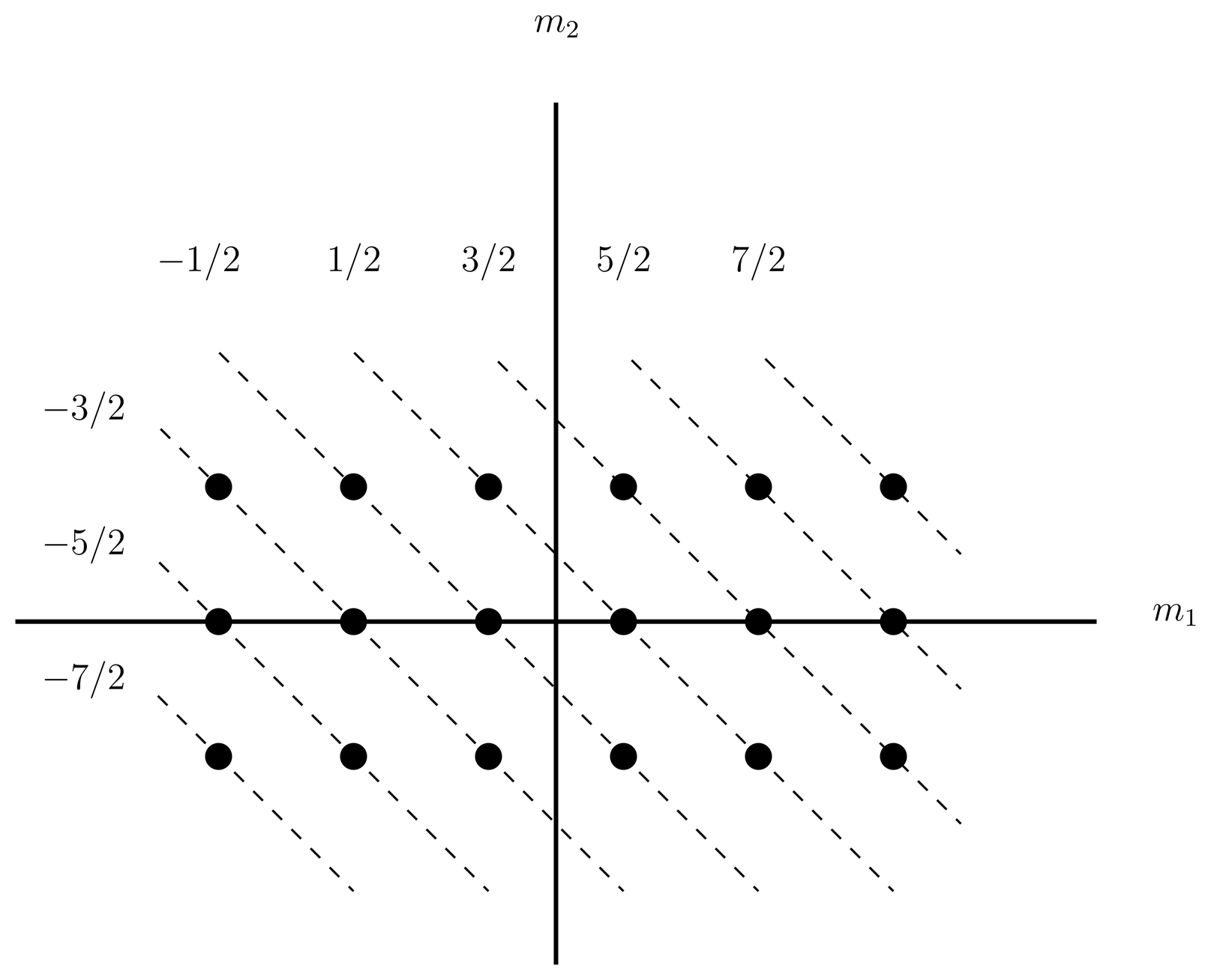
Each dot in the rectangular array stands for one vector of the uncoupled or tensor product basis, \ket{j_1j_2m_1m_2} = \ket{j_1m_1}\ket{j_2m_2}. The dashed lines are contours of m=m_1+m_2. — Figure 1:Each dot in the rectangular array stands for one vector of the uncoupled or tensor product basis, $\ket{j_1j_2m_1m_2} = \ket{j_1m_1}\ket{j_2m_2}$ . The dashed lines are contours of $m=m_1+m_2$ .

These eigenvalues of $J_z$ are in general degenerate. To follow the subsequent argument, it helps to have an example. Let us take the case $j_1=\frac{5}{2}$ and $j_2=1$ , so that $2j_1+1=\dim\ES_1=6$ and $2j_2+1=\dim\ES_2=3$ . Thus, the dimensionality of $\ES=\ES_1\otimes\ES_2$ is $6\times3=18$ . It is convenient to make a plot in the $m_1$ - $m_2$ plane of the basis vectors of the tensor product basis, by placing a dot at each allowed $m_1$ and $m_2$ value. We then obtain a rectangular array of dots, as illustrated in Figure 1. As illustrated in the figure, lines of constant $m=m_1+m_2$ are straight lines, dashed in the figure, sloping downwards. The number of dots each dashed line passes through is the number of kets of the uncoupled basis with a given $m$ value; we see that the degeneracies of the different $m$ values range from one to three, as summarized in Table~jjcouple-1.

In particular, the stretched state (the one for which $(m_1,m_2) = (j_1,j_2)$ , in the upper right hand corner in the figure) is a nondegenerate eigenstate of $J_z$ with quantum number $m=\frac{7}{2}$ . But since $[J^2,J_z]=0$ , this state is also an eigenstate of $J^2$ , in accordance with Theorem Theorem. But what is the eigenvalue of $J^2$ , that is, what is the quantum number $j$ ? Certainly we cannot have $j<\frac{7}{2}$ , because then this would violate the rule $m\le j$ . Nor can we have $j>\frac{7}{2}$ , because, for example, if the stretched state were $\ket{jm} = \ket{\frac{9}{2} \frac{7}{2}}$ , then we could apply the raising operator $J_+$ and obtain the state $\ket{\frac{9}{2}\frac{9}{2}}$ . But there is no state with $m=\frac{9}{2}$ , as we see from the figure or table. Therefore the $j$ quantum number of the stretched state must be $j=\frac{7}{2}$ ; this state is the state $\ket{jm} = \ket{\frac{7}{2}\frac{7}{2}}$ of the coupled basis. But given this state, we can apply lowering operators $J_-$ to obtain all eight states $\ket{\frac{7}{2} m}$ , which are indicated in the third column of the table.

{\tiny\singlespacing\bf Table~jjcouple-1. \rm The first column contains $m$ , the quantum number of $J_z$ ; the second column contains $g(m)$ , the degeneracy of $m$ ; columns 3, 4 and 5 contain a unit for each vector $\ket{jm}$ of the standard or coupled basis with given $j$ and $m$ values.}

Now let us consider the 2-dimensional eigenspace of $J_z$ corresponding to quantum number $m=\frac{5}{2}$ . This space is spanned by the kets of the uncoupled basis corresponding to $(m_1,m_2) = (\frac{5}{2},0)$ and $(\frac{3}{2}, 1)$ . Furthermore, the ket $\ket{\frac{7}{2}\frac{5}{2}}$ of the coupled basis also lies in this space. Let us consider the ket, call it $\ket{x}$ , that is orthogonal to $\ket{\frac{7}{2}\frac{5}{2}}$ in this space. Certainly $\ket{x}$ is an eigenket of $J_z$ with eigenvalue $\frac{5}{2}$ . And it is also an eigenket of $J^2$ , a fact that is left as an exercise (the logic is an extension of the proof of Theorem Theorem). But what is the $j$ value? Certainly we cannot have $j<\frac{5}{2}$ , because this would violate the $m\le j$ rule. Nor can we have $j>\frac{5}{2}$ , because if we had $j=\frac{7}{2}$ , for example, for the state $\ket{x}$ , then we would have two linearly independent states, both with $m=\frac{5}{2}$ and $j=\frac{7}{2}$ . We could then apply the raising operator $J_+$ to both of them, and obtain two linearly independent states with $m=\frac{7}{2}$ , $j=\frac{7}{2}$ . But there is only one state with $m=\frac{7}{2}$ , as we see from the figure or table. Therefore we must have $j=\frac{5}{2}$ for the state $\ket{x}$ , which otherwise is the ket $\ket{\frac{5}{2}\frac{5}{2}}$ of the coupled basis. Then, by applying lowering operators to this, we obtain all six vectors $\ket{\frac{5}{2} m}$ , which are indicated in the fourth column of the table. Finally, we carry out the same procedure for the 3-dimensional space corresponding to $m=\frac{3}{2}$ , and we obtain four more vectors $\ket{\frac{3}{2} m}$ of the coupled basis.

In this way, all 18 dimensions of $\ES$ are used up, as indicated by the totals at the bottom of the table. We see that the tensor product space $\ES$ consists of the direct sum of three irreducible subspaces, corresponding to $j=\frac{3}{2}$ , $\frac{5}{2}$ , and $\frac{7}{2}$ , and that each of these $j$ values occurs with multiplicity one. These facts are summarized by the notation,

\frac{5}{2} \otimes 1 = \frac{3}{2} \oplus \frac{5}{2} \oplus \frac{7}{2},

(46)

which corresponds to the dimensionality count,

18 =6\times3 = 4 + 6 + 8.

(47)

By using diagrams like these, it is easy to work out the general case in which we combine arbitrary angular momenta $j_1$ and $j_2$ . The result is

j_1 \otimes j_2 = |j_1 - j_2| \oplus |j_1-j_2|+1 \oplus \dots \oplus j_1+j_2,

(48)

that is, the $j$ values in $j_1\otimes j_2$ range from a minimum of $|j_1-j_2|$ to a maximum of $j_1+j_2$ in integer steps, and each $j$ value in this range occurs once. Since no $j$ value occurs more than once, there is no need for the index $\gamma$ , and the vectors of the coupled basis can be denoted simply $\ket{jm}$ . Also, since the dimensionalities of the subspaces must add up to the dimensionality of the tensor product space, we have the identity

\sum_{j=|j_1-j_2|}^{j_1+j_2} 2j+1 = (2j_1+1)(2j_2+1).

(49)

This identity can be proved by elementary algebra, as a check on the count of dimensions.

The Clebsch-Gordan Coefficients¶

At this point we have two bases in $\ES=\ES_1\otimes\ES_2$ , the uncoupled basis $\ket{j_1j_2m_1m_2}$ with $-j_1 \le m_1 \le j_1$ and $-j_2 \le m_2 \le j_2$ and the coupled basis $\ket{jm}$ with $|j_1-j_2| \le j \le j_1+j_2$ and $-j \le m \le j$ . These two bases must be connected by a unitary matrix, the components of which are just the scalar products of the vectors from one basis with the vectors from the other. That is, we have

\begin{aligned} \ket{jm} &= \sum_{m_1=-j_1}^{j_1} \sum_{m_2=-j_2}^{j_2} \ket{j_1j_2m_1m_2} \braket{j_1j_2m_1m_2}{jm}, \end{aligned}

(50)

\begin{aligned} \ket{j_1j_2m_1m_2} &= \sum_{j=|j_1-j_2|}^{j_1+j_2} \sum_{m=-j}^j \ket{jm}\braket{jm}{j_1j_2m_1m_2}, \end{aligned}

(51)

which can be regarded as the insertion of two resolutions of the identity in two different ways. The expansion coefficients $\braket{j_1j_2m_1m_2}{jm}$ or $\braket{jm}{j_1j_2m_1m_2}$ are called the Clebsch-Gordan coefficients or the vector coupling coefficients. Note the effect of the selection rule (56) on the sums (50): many of the terms are zero.

The Clebsch-Gordan coefficients are determined by (50) only to within certain phase conventions. As explained in Phase Conventions and Matrix Elements of $J_\pm$ , the relative phases of the basis vectors $\ket{jm}$ inside a given irreducible subspace are chosen so that the matrix elements of $J_+$ and $J_-$ are real and positive, but this still leaves arbitrary the phases of the stretched states within each irreducible subspace. This in turn leaves some arbitrariness in the phase conventions for the Clebsch-Gordan coefficients. These are pinned down by a further phase convention,

\braket{jj}{j_1j_2j_1,j-j_1} > 0,

(52)

for each allowed $j$ value in $j_1\otimes j_2$ , which is due to Condon and Shortley, authors of the classic book The Theory of Atomic Spectra. Under these phase conventions, the Clebsch-Gordan coefficients are real, that is,

\braket{jm}{j_1j_2m_1m_2} =\braket{j_1j_2m_1m_2}{jm},

(53)

so that the unitary matrix connecting the coupled and uncoupled bases is in fact a real, orthogonal matrix.

The Clebsch-Gordan coefficients have several properties that follow in a simple way from their definition. The first follows from the fact that the Clebsch-Gordan coefficients are the components of a unitary matrix, so that

\begin{aligned} \sum_{m_1m_2} \braket{jm}{j_1j_2m_1m_2} \braket{j_1j_2m_1m_2}{j'm'} &= \delta_{jj'} \, \delta_{mm'}, \end{aligned}

(54)

\begin{aligned} \sum_{jm} \braket{j_1j_2m_1m_2}{jm} \braket{jm}{j_1j_2m'_1m'_2} &= \delta_{m_1m'_1} \, \delta_{m_2m'_2}. \end{aligned}

(55)

Again, these are nothing but orthonormality relations for the two bases, with resolutions of the identity inserted.

Another property is the selection rule,

\braket{jm}{j_1j_2m_1m_2} = 0 \quad \\textunless m=m_1+m_2,

(56)

which follows immediately from (44).

The Clebsch-Gordan coefficients also satisfy various recursion relations. We can obtain one of these by applying $J_- = J_{1-} +J_{2-}$ to (50). This gives

\begin{aligned} {1\over\hbar} J_-\ket{jm} &= \sqrt{(j+m)(j-m+1)} \, \ket{j,m-1} \end{aligned}

(57)

\begin{aligned} &= \sum_{m_1m_2} \Bigl( \sqrt{(j_1+m_1)(j_1-m_1+1)} \, \ket{j_1j_2,m_1-1,m_2} \end{aligned}

(58)

\begin{aligned} \quad &+ \sqrt{(j_2+m_2)(j_2-m_2+1)} \, \ket{j_1j_2m_1,m_2-1} \Bigr) \braket{j_1j_2m_1m_2}{jm} \end{aligned}

(59)

\begin{aligned} &=\sum_{m_1m_2} \Bigl( \sqrt{(j_1-m_1)(j_1+m_1+1)} \, \braket{j_1j_2,m_1+1,m_2}{jm} \end{aligned}

(60)

\begin{aligned} & +\sqrt{(j_2-m_2)(j_2+m_2+1)}\, \braket{j_1j_2m_1,m_2+1}{jm} \Bigr) \end{aligned}

(61)

\begin{aligned} &\qquad \times \ket{j_1j_2m_1m_2}, \end{aligned}

(62)

to which we apply the bra $\bra{j_1j_2m'_1m'_2}$ from the left and rearrange indices to obtain,

\begin{aligned} &\sqrt{(j+m)(j-m+1)}\, \braket{j_1j_2m_1m_2}{j,m-1} \\ &\qquad=\sqrt{(j_1-m_1)(j_1+m_1+1)} \, \braket{j_1j_2,m_1+1,m_2}{jm} \\ &\qquad+\sqrt{(j_2-m_2)(j_2+m_2+1)} \, \braket{j_1j_2m_1,m_2+1}{jm}. \\ \end{aligned}

(63)

Similarly, working with $J_+$ we obtain,

\begin{aligned} &\sqrt{(j-m)(j+m+1)}\,\braket{j_1j_2m_1m_2}{j,m+1} \\ &\qquad=\sqrt{(j_1+m_1)(j_1-m_1+1)}\, \braket{j_1j_2,m_1-1,m_2}{jm} \\ &\qquad+\sqrt{(j_2+m_2)(j_2-m_2+1)} \, \braket{j_1j_2m_1,m_2-1}{jm}. \\ \end{aligned}

(64)

The method of Calculating the Clebsch-Gordan Coefficients for calculating the Clebsch-Gordan coefficients uses a slightly disguised version of these recursion relations.

Other properties of the Clebsch-Gordan coefficients include the following identities:

\begin{aligned} \braket{j_1j_2m_1m_2}{jm} &= (-1)^{j_1+j_2-j} \braket{j_2j_1m_2m_1}{jm}, \end{aligned}

(65)

\begin{aligned} &=(-1)^{j_1-j+m_2} \sqrt{{\ds 2j+1 \over \ds 2j_1+1}} \, \braket{jj_2m,-m_2}{j_1m_1}, \end{aligned}

(66)

\begin{aligned} &= (-1)^{j_2-j-m_1} \sqrt{{\ds 2j+1 \over \ds 2j_2+1}} \, \braket{j_1j,-m_1,m}{j_2m_2}, \end{aligned}

(67)

\begin{aligned} &= (-1)^{j_1+j_2-j} \braket{j_1j_2,-m_1,-m_2}{j,-m}. \end{aligned}

(68)

We will not prove these identities here. If you ever have to use such identities in a serious way, you should look into the Wigner $3j$ -symbols, which provide a more symmetrical way of dealing with Clebsch-Gordan coefficients.

Calculating the Clebsch-Gordan Coefficients¶

The following method for calculating the Clebsch-Gordan coefficients differs slightly from the usual one taught in introductory courses, mainly in its method of handling the stretched states. We illustrate it with the example of Allowed Values of $j$ and $m$ , in which $j_1=\frac{5}{2}$ and $j_2=1$ . Suppose we wish to obtain the Clebsch-Gordan coefficient $\braket{j_1j_2m_1m_2}{jm}=\braket{\frac{5}{2} 1 \frac{1}{2} 0}{\frac{3}{2}\frac{1}{2}}$ . We begin by writing $\ket{jm}=\ket{\frac{3}{2}\frac{3}{2}}$ , the stretched state in the irreducible subspace $j=\frac{3}{2}$ , as a linear combination of basis vectors of the uncoupled basis with $m=m_1+m_2=\frac{3}{2}$ :

\ket{\frac{3}{2}\frac{3}{2}} = a\ket{\frac{5}{2}}\ket{-1} + b\ket{\frac{3}{2}}\ket{0} + c\ket{\frac{1}{2}}\ket{1},

(69)

where $\ket{m_1}\ket{m_2}$ is short for $\ket{j_1m_1}\ket{j_2m_2}$ and where $a$ , $b$ and $c$ are the expansion coefficients. We determine these by applying $J_+ = J_{1+}+J_{2+}$ to both sides. The left hand side is annihilated by $J_+$ so we obtain

\begin{aligned} 0&= a\bigl[(J_{1+}\ket{\frac{5}{2}})\ket{-1}+ \ket{\frac{5}{2}}(J_{2+}\ket{-1})\bigr] +b\bigl[(J_{1+}\ket{\frac{3}{2}})\ket{0} + \ket{\frac{3}{2}}(J_{2+}\ket{0})\bigr] \\ &\qquad +c\bigl[(J_{1+}\ket{\frac{1}{2}})\ket{1} + \ket{\frac{1}{2}}(J_{2+}\ket{1})\bigr] \\ &=a\bigl[0 + \sqrt{2}\ket{\frac{5}{2}}\ket{0}\bigr] + b\bigl[\sqrt{5}\ket{\frac{5}{2}}\ket{0} + \sqrt{2}\ket{\frac{3}{2}}\ket{1}\bigr] +c\bigl[\sqrt{8}\ket{\frac{3}{2}}\ket{1}+0\bigr], \\ \end{aligned}

(70)

or, since the basis vectors are linearly independent,

\sqrt{2}\,a + \sqrt{5}\,b=0, \qquad \sqrt{2}\,b + \sqrt{8}\,c=0.

(71)

This determines the vector $(a,b,c)$ to within a normalization and phase. By (69) this vector must be normalized, and by (52) $a$ is real and positive. Taken together, these imply,

\ket{\frac{3}{2}\frac{3}{2}} = \sqrt{\frac{2}{3}}\,\ket{\frac{5}{2}}\ket{-1} -{2\over\sqrt{15}}\,\ket{\frac{3}{2}}\ket{0} +\sqrt{\frac{1}{15}}\,\ket{\frac{1}{2}}\ket{1}.

(72)

This is the stretched state in the $j=\frac{3}{2}$ subspace. Notice that we did not have to go through the Clebsch-Gordan coefficients for $j=\frac{7}{2}$ or $\frac{5}{2}$ to obtain it.

We now apply $J_-=J_{1-}+J_{2-}$ to both sides. On the left we obtain $\sqrt{3}\ket{\frac{3}{2}\frac{1}{2}}$ , while the right hand side can be expressed as a linear combination of the vectors of the uncoupled basis. The result is

\ket{\frac{3}{2}\frac{1}{2}} = \sqrt{\frac{2}{5}}\ket{\frac{3}{2}}\ket{-1} -\sqrt{\frac{2}{5}}\ket{\frac{1}{2}}\ket{0} +\sqrt{\frac{1}{5}}\ket{-\frac{1}{2}}\ket{1}.

(73)

The desired Clebsch-Gordon coefficient can be read off from this,

\braket{\frac{5}{2} 1 \frac{1}{2} 0}{\frac{3}{2}\frac{1}{2}} =-\sqrt{\frac{2}{5}}.

(74)

This method is suitable for calculating Clebsch-Gordan coefficients by hand for small quantum numbers. There are also explicit formulas for the Clebsch-Gordan coefficients. These are awkward to use for calculation by hand, but are easily coded into computer programs. See also the link to the table of Clebsch-Gordan coefficients.

Universal Coefficients and Matrices¶

The Clebsch-Gordan coefficients have been constructed in such a way that they depend only on the angular momentum commutation relations and various phase conventions for the standard angular momentum basis states. They do not depend on the physical interpretation of the angular momenta that occur ( $\Jvec_1$ , $\Jvec_2$ , $\Jvec=\Jvec_1+\Jvec_2$ , etc., whether spin, orbital, isospin, or any other kind), or on the nature of the vector space upon which these operators act (whether a state space for a quantum mechanical system or any other kind). The Clebsch-Gordan coefficients are just numbers that are universal in the sense that they apply in the analysis of any physical system, as long as the standard phase and other conventions are followed.

Therefore the scalar product that appears in the notation $\braket{jm}{j_1j_2m_1m_2}$ for the Clebsch-Gordan coefficient can be understood as taking place in some model space, one that is set up just for the purposes of constructing the coefficients. It is not necessarily the same as the state space for whatever application one is making. For this reason some authors prefer to write the Clebsch-Gordan coefficients as $C^{jm}_{j_1j_2m_1m_2}$ or some such notation, to avoid confusing the scalar products in the two different spaces. The scalar product notation used in these notes has the advantage that it makes identities such as (50) obvious.

Similar considerations apply to the $D$ -matrices. According to the definition (58), these are the components of rotation operators with respect to a standard angular momentum basis. The matrices that result are independent of the nature of the space upon which the matrix elements are taken, as long as standard conventions are followed for the phases etc.{} of the basis vectors. Therefore the $D$ -matrices are universal in the sense that they apply in all physical applications, as long as standard conventions are followed. The space in which the matrix element is taken in the definition (58) can be any model space in which the standard conventions are followed.

Rotations, $D$ -matrices and Clebsch-Gordan Coefficients¶

Let us now consider the effect of the rotation operator $U({\hat{\mathbf{n}}},\theta)$ on the tensor product space $\ES=\ES_1\otimes\ES_2$ . This rotation operator is defined in the usual way, and can be expressed in terms of the rotation operators $U_1({\hat{\mathbf{n}}},\theta)$ and $U_2({\hat{\mathbf{n}}},\theta)$ that act on the constituent spaces $\ES_1$ and $\ES_2$ :

\begin{aligned} U({\hat{\mathbf{n}}},\theta) &= e^{-i\theta{\hat{\mathbf{n}}}\cdot\Jvec/\hbar} = e^{-i\theta{\hat{\mathbf{n}}}\cdot(\Jvec_1+\Jvec_2)/\hbar} \end{aligned}

(75)

\begin{aligned} &= e^{-i\theta{\hat{\mathbf{n}}}\cdot\Jvec_1/\hbar} e^{-i\theta{\hat{\mathbf{n}}}\cdot\Jvec_2/\hbar} =U_1({\hat{\mathbf{n}}},\theta)U_2({\hat{\mathbf{n}}},\theta). \end{aligned}

(76)

Here the exponential of the sum factors into a product of exponentials because $\Jvec_1$ and $\Jvec_2$ commute.

Interesting results can be obtained from this. First let us apply a rotation operator $U$ to a vector of the uncoupled basis. We find

\begin{aligned} U\ket{j_1j_2m_1m_2} &= (U_1 \ket{j_1m_1}) (U_2\ket{j_2m_2}) =\sum_{m'_1m'_2} \ket{j_1j_2m'_1m'_2} D^{j_1}_{m'_1m_1} D^{j_2}_{m'_2m_2} \end{aligned}

(77)

\begin{aligned} &= \sum_{jm} \sum_{m'} \ket{jm'} D^j_{m'm} \braket{jm}{j_1j_2m_1m_2}, \end{aligned}

(78)

where we use (91) and (51), and where it is understood that all $D$ matrices have the same axis and angle $({\hat{\mathbf{n}}},\theta)$ . Then we multiply this on the left by $\bra{j_1j_2m''_1m''_2}$ and rearrange indices, to obtain,

D^{j_1}_{m_1m'_1} D^{j_2}_{m_2m'_2} = \sum_{jmm'} \braket{j_1j_2m_1m_2}{jm} D^j_{mm'} \braket{jm'}{j_1j_2m'_1m'_2}.

(79)

In a similar manner we can obtain the identity,

D^j_{mm'} = \sum_{\begin{matrix}\scriptstyle m_1m_2 \\ \scriptstyle m'_1m'_2\\\end{matrix}} \braket{jm}{j_1j_2m_1m_2} D^{j_1}_{m_1m'_1} D^{j_2}_{m_2m'_2} \braket{j_1j_2m'_1m'_2}{jm'}.

(80)

These identities are useful for a variety of purposes; for example, (79) can be used whenever it is necessary to express a product of $D$ matrices as a linear combination of single $D$ matrices (a problem that arises often in atomic, molecular, and nuclear physics), and (80) shows that $D$ matrices for small values of $j$ can be combined to find the $D$ matrices for larger values of $j$ .

The Three- $Y_{\ell m}$ Formula¶

We present here one application of (79), in which we use (68) to obtain an identity involving the $Y_{\ell m}$ 's. First we change notation in (79), setting $j_1=\ell_1$ , $j_2=\ell_2$ and $j=\ell$ (indicating integer angular momenta), and we set $m'_1=m'_2=0$ . Then because of the selection rule (56), the $m'$ sum on the right hand side is replaced by the single term $m'=0$ . Then we take the complex conjugate of both sides and use (68), to obtain

\begin{aligned} Y_{\ell_1m_1}(\theta,\phi) Y_{\ell_2m_2}(\theta,\phi) &= \sum_{\ell m} \sqrt{\ds{\ds(2\ell_1+1)(2\ell_2+1) \over \ds 4\pi(2\ell+1)}} \end{aligned}

(81)

\begin{aligned} & \quad \times Y_{\ell m}(\theta,\phi)\, \braket{\ell m}{\ell_1\ell_2m_1m_2} \braket{\ell_1\ell_2 00}{\ell 0}. \end{aligned}

(82)

Of course, the product of two $Y_{\ell m}$ 's is a function on the unit sphere, which can be expanded as a linear combination of other $Y_{\ell m}$ 's; this formula gives the expansion explicitly. We see that the $\ell$ values that contribute are exactly those which occur in $\ell_1\otimes\ell_2$ . Finally, we can multiply this by $Y^\cc_{\ell_3m_3}$ and integrate to obtain the useful formula,

\int d\Omega \, Y^\cc_{\ell_3m_3} Y_{\ell_1m_1} Y_{\ell_2m_2} = \sqrt{\ds{\ds(2\ell_1+1)(2\ell_2+1) \over \ds 4\pi(2\ell_3+1)}} \, \braket{\ell_3m_3}{\ell_1\ell_2m_1m_2} \braket{\ell_1\ell_2 0 0}{\ell_3 0}.

(83)

We will call this the *three- $Y_{\ell m*}$ formula}; it is very useful in atomic physics. This formula and (79) can be regarded as a special cases of the Wigner-Eckart theorem, which we consider later.

In conclusion, we mention a special case of (82), obtained by setting $m_1=m_2=0$ and using (51),

P_{\ell_1}(\cos\theta)P_{\ell_2}(\cos\theta) = \sum_\ell P_\ell(\cos\theta)\, |\braket{\ell0}{\ell_1\ell_200}|^2,

(84)

which is sometimes useful.

Problems¶

Problem 1.

About wave functions of particles, including spin.

(a) The wave function of a particle with spin was defined in (14). If $\psi_m(\rvec)$ is the wave function of a spinning particle in state $\ket{\psi}$ , then what is the wave function of the particle in the rotated state, $U(\Rmat)\ket{\psi}$ ? The rotation operator $U(\Rmat)$ is the product of a spatial rotation times a spin rotation, both parameterized by the same $\Rmat$ .

(b) Let us use the Pauli equation to describe the dynamics of an electron. The wave function is a 2-component spinor as in (16), and in the Pauli Hamiltonian (29) we set $q=-e$ and $g=g_e$ , the electron $g$ -factor. Also note the sign in (16), that is, $\muvec=-g_e\mu_B(\Svec/\hbar)$ , which comes from the fact that the charge on the electron is negative.

Consider an electron in a central force potential $V(r)$ , plus a uniform magnetic field $\Bvec = B {\hat{\mathbf{b}}}$ . Let $\omega_0 = eB/mc$ . Use the gauge $\Avec = \frac{1}{2} \Bvec \cross \rvec$ . Consider the time-dependent Pauli equation for the electron,

i\hbar\pop{}{t} \ket{\psi(t)} = H\ket{\psi(t)},

(85)

where $H$ is the Pauli Hamiltonian (29) and where $q\Phi = V(r)$ .

Define a new state $\ket{\phi(t)}$ by

\ket{\psi(t)} = U({\hat{\mathbf{b}}},\omega t) \ket{\phi(t)},

(86)

where $U({\hat{\mathbf{b}}},\omega t)$ is a rotation operator that rotates the whole system (orbital and spin degrees of freedom). This means that $\ket{\phi(t)}$ is the state in a frame rotating with angular velocity $\omega$ about the axis ${\hat{\mathbf{b}}}$ .

Find a frequency $\omega$ that eliminates the effect of the magnetic field on the orbital motion of the particle, apart from the centrifugal potential which is proportional to $(\bvec \cross \rvec)^2$ . Find a frequency $\omega$ that eliminates the effect of the magnetic field on the spin. Express your answers as some multiple of $\omega_0$ . Can you eliminate the effects of the magnetic field entirely, apart from the centrifugal potential?

Problem 2.

In Notes~\magfield{} we worked out the energy levels of a ``spinless electron’’ in a uniform magnetic field. Including the spin, find the energy levels of an electron in a uniform magnetic field. You may approximate $g\approx 2$ . Express your answer in terms of $\omega_0 = eB/mc$ , the orbital frequency of a classical electron in a uniform magnetic field. Sketch the first few Landau energy levels on a vertical energy axis, first in the model in which we ignore the electron spin, and then after we take the spin into account. Ignore the energy coming from the $z$ -motion in this diagram. Label the levels by their degeneracies. What happens if you take into account the fact that $g$ is not exactly 2? This is a short problem, and does not require any lengthy calculations.

Problem 3.

I won’t ask you to work out any numerical values of Clebsch-Gordan coefficients, but you should be comfortable in doing so. The following is a related problem.

Consider the angular momentum problem $\ell \otimes \frac{1}{2}$ , where $\ell$ is arbitrary and could be very large. We write $j=\ell+\frac{1}{2}$ or $j=\ell-\frac{1}{2}$ for the resulting angular momentum. By beginning with the doubly stretched state,

\ket{\ell+\frac{1}{2},\ell+\frac{1}{2}} = \ket{\ell \ell} \ket{\frac{1}{2} \frac{1}{2}},

(87)

apply lowering operators to construct the states $\ket {\ell +\frac{1}{2},m}$ for $m$ going down to $\ell-\frac{5}{2}$ . By this time a pattern should be evident; guess it, and prove that it is right by induction, to obtain a general formula for $\ket{\ell+\frac{1}{2},m}$ . You may simplify notation by omitting the total angular momenta $\ell$ and $\frac{1}{2}$ in the kets on the right hand sides of your equations, because they are always the same; for example, the right hand side of (87) can be written simply $\ket{\ell}\ket{\frac{1}{2}}$ .

Now construct the stretched state for $j=\ell-\frac{1}{2}$ , namely $\ket{\ell-\frac{1}{2},\ell-\frac{1}{2}}$ . Use the standard phase convention given by (52). Then lower this enough times to see a pattern, guess it, and prove it by induction.

The following are some useful formulas that can be derived by the methods of this problem. We present them here for future reference. We combine $\ell\otimes 1$ , and find, for the three cases $j=\ell+1$ , $j=\ell$ , and $j=\ell-1$ , the following:

\begin{aligned} &\ket{\ell+1,m} = \sqrt{(\ell+m+1)(\ell+m) \over (2\ell+2)(2\ell+1)}\, \ket{m-1}\ket{1} &+\sqrt{(\ell-m+1)(\ell+m+1) \over (\ell+1)(2\ell+1)} \, \ket{m}\ket{0} +\sqrt{(\ell-m)(\ell-m+1) \over (2\ell+2)(2\ell+1)} \, \ket{m+1}\ket{-1}. \end{aligned}

(88)

\begin{aligned} &\ket{\ell m} = -\sqrt{(\ell-m+1)(\ell+m) \over 2\ell(\ell+1)} \, \ket{m-1}\ket{1} &+{m \over \sqrt{\ell(\ell+1)}} \ket{m}\ket{0} +\sqrt{(\ell-m)(\ell+m+1) \over 2\ell(\ell+1)} \, \ket{m+1}\ket{-1}. \end{aligned}

(89)

\begin{aligned} &\ket{\ell-1,m} = \sqrt{(\ell-m)(\ell-m+1) \over 2\ell(2\ell+1)} \, \ket{m-1}\ket{1} &-\sqrt{(\ell-m)(\ell+m) \over \ell(2\ell+1)}\, \ket{m}\ket{0} +\sqrt{(\ell+m+1)(\ell+m) \over 2\ell(2\ell+1)}\, \ket{m+1}\ket{-1}. \end{aligned}

(90)