35. The Photoelectric Effect
Introduction
In these notes we consider the ejection of an atomic electron by an incident photon, which is an example of the photoelectric effect. The photon should have an energy in the ultraviolet to x-ray range, for reasons to be explained below; thus, our results will provide a semi-quantitative model for the absorption of x-rays by matter. In these notes, we use a version of the semiclassical theory of radiation, in which the radiation field is treated classically, but the atomic system quantum mechanically. Certain quantum mechanical concepts, notably photons, are used in the description of the classical radiation field. The photoelectric effect is not only interesting and important physically, but the following calculation also provides excellent exercise in time-dependent perturbation theory, the treatment of cross s, and assorted physical facts.
The Incident Photon
We suppose the incident photon has energy and momentum . (We use the 0 subscript to refer to the incident photon; quantities without this subscript, such as or , will refer to the ejected electron.) For simplicity, we assume the atom has a single electron (or a single electron of interest), and that it is initially in its ground state. We let be the energy of this ground state; naturally, . Then by conservation of energy, we must have
so that the photon will have enough energy to eject the electron.
Actually, we will make a stronger assumption, namely,
for the following reason. Assuming the atom is initially neutral, the ejected electron leaves a positive ion behind and travels out in the long-range Coulomb field of the ion. Therefore the final electron state is not that of a free particle, but rather one of the unbound or positive energy solutions of the Coulomb potential. The unbound Coulomb wave functions are important in many applications, and they can be determined by the usual methods for solving differential equations (power series, etc). These wave functions turn out to be hypergeometric functions, and for serious work involving Coulomb scattering and other applications one must know about them. Nevertheless, it would be simpler if we could deal with free particle wave functions for the final electron states. We can do this in a certain approximation if we assume that the energy of the ejected electron is much greater than the binding energy , so that the ejected electron does not feel the Coulomb field very much. This is why we make the assumption (2), so that we can approximate the final electron wave functions by free particle solutions.
By energy conservation we have
where is the final electron energy. Under the condition (2), both and will be large compared to , and nearly equal to one another. Therefore we can rewrite the condition (2) in another form, and combine it with the condition that our electron be nonrelativistic, by writing
This can be put into dimensionless form by dividing by ,
where we use the estimate , valid for hydrogen-like atoms. For example, in the case of hydrogen, we might restrict the energy of the incident photon to lie in the range,
Such photons lie in the far ultraviolet to x-ray region. If we were willing to deal with hypergeometric functions we could extend the lower limit downward; if we were willing to use relativistic quantum mechanics, we could extend the upper limit upwards. But we will live with the stated limits.
We will describe the incident photon by means of a classical light wave, with vector potential
where is the amplitude (assumed to be real), and where is the polarization unit vector (also assumed to be real, indicating linear polarization). This vector potential is in the Coulomb gauge (the scalar potential is taken to be zero), so that
as follows by taking the divergence of (7) and using the transversality condition,
The Atomic System
The atomic system for the one-electron atom described by the unperturbed Hamiltonian,
For part of the following calculation we can leave unspecified, but at a certain point we will specialize to a hydrogen-like atom with
As mentioned, we assume that the atom is initially in its ground state with energy , so that
We will assume that the unbound electron in the final state is described by a plane wave with wave vector ,
where we adopt box normalization as in (68)--(70). The final energy is denoted .
The perturbing Hamiltonian is
which comes from expanding and dropping the term in . We note that because of the Coulomb gauge condition (8). We will also write the perturbing Hamiltonian in the form,
[see (43)], so that
We drop the term in because we will be working only to first order in perturbation theory; if we were to go to second order, this term would have to be included.
The Transition Rate
We can now proceed to the transition rate, which follows from (47) and which we write in the form,
where
The sum in (17) is to be taken over final states which lie in a small cone of solid angle about some final wave vector , as in Fig.~\figr\tdpt.5. We choose the direction of to be some direction of interest, and we choose the magnitude of by conservation of energy, so that
The notational difference between and is that is a variable final electron state over which we are summing, which does not necessarily conserve energy, while does conserve energy and is in some fixed direction of interest.
Next we make the replacement
and the replacement (81) in (17), in order to go over to the transition rate per unit solid angle. This gives
which we will transform in various ways. First we must relate to the differential cross ,
where is the number density of the incident particles and is their velocity. But since the incident particles are photons, their velocity is .
To compute we must mix classical and quantum concepts. An incident beam consisting of photons per unit volume has an energy density ; on the other hand, by classical electromagnetic theory we have . In the light wave (7) the electric and magnetic contributions to the energy density are equal, and cross terms vanish when we average over the volume of the box. Thus we find,
or
where we have used . We now solve (22) for the cross , finding,
The Matrix Element and Cross Section
Next we work on the right hand side of (21). First, we write out the matrix element, using (16),
where in the final step we have allowed the momentum operator to act to the left on the plane wave state , bringing out a factor of . The remaining matrix element can be expressed in terms of the Fourier transform of the ground state wave function ,
where
and where
Finally, we transform the function in (21), using (18) and (19):
At this point we remark that had we been doing a problem in the emission or absorption of optical radiation from an atom, we would have been able to expand the exponential in (26), since radiation in this frequency range satisfies (the wavelength is much larger than the atomic size). This would lead to the multipole expansion (the dipole approximation at lowest order). We cannot make this expansion in the present calculation, however, because we are dealing with radiation of short wavelength, such as x-rays.
We now gather all the pieces together [(25), (21), (26), (27) and (30)] to obtain
or,
where now . We see that all the volume factors cancel out of (31), as they should, as do the factors of , which we expect because a cross by definition is independent of the incident flux. The vector reminds us of the momentum transfer vector which occurred in our analysis of elastic scattering in 34. Time-Dependent Perturbation Theory, but here the quantity is the momentum difference between the final electron and the initial photon. Unlike the case of elastic scattering, where we had , here the vectors and are of different magnitudes.
Momentum Transfer
The fact that the vector is nonzero means that a proper understanding of momentum conservation must take into account the nucleus as well as the photon and the electron. The reason the nuclear momentum has not appeared explicitly in our calculations is that we implicitly assumed in writing down (10) that the nuclear mass was infinitely large in comparison to the electron mass. This of course is a good approximation, and it means that the nucleus can carry off a large amount of momentum without moving very fast. In the limit of infinite nuclear mass, the nucleus acts like a momentum source or sink which is able to provide whatever momentum is needed for the reaction at hand. This is important, because in the absence of such a momentum source, a reaction such as
that is, the absorption of a photon by a free electron, is impossible (one cannot satisfy both energy and momentum conservation in this reaction). Similarly, in the absence of a momentum source, the reaction
is impossible. But if there is a nucleus nearby to take up some momentum, then the reaction (34) does occur; this is called Bremsstrahlung (German for “braking radiation”), and it is one of the principal mechanisms for the slowing down of fast charged particles in matter (especially important for light particles like electrons and muons). Our assumption of infinite nuclear mass in the present calculation has caused the conservation of momentum to appear only implicitly, in contrast to the conservation of energy, which is explicitly expressed by the -function in (31).
We have written the cross (32) so that the classical radius of the electron makes its appearance,
This radius is called classical because there is no in it; its physical meaning is that it is the radius (to within an order of magnitude) outside of which the electrostatic energy of the nominal monopole field (divided by ) equals the mass of the electron. The total electrostatic energy in the field of a monopole is, of course, infinite.
To proceed with the analysis, we will now assume that , for a hydrogen-like atom. Then the ground state wave function is
where and is the usual Bohr radius. It is then straightforward to compute the Fourier transform, according to (29). We find
This is obviously proportional to the momentum-space wave function of the ground state of the hydrogen atom; notice that it is a rational function of the momentum. In any case, the cross now becomes
Approximating the Cross Section
This cross can be boiled down further by incorporating the approximation (4). This occurs in two steps. First, it turns out that the initial photon wave number is much smaller than the final electron wave number . To show this, we write out the conservation of energy equation (3) in the form
where we neglect in comparison to . But this can be put in the form,
where and are the final electron momentum and velocity, respectively, and where we make use of the nonrelativistic assumption . We see that is indeed small, of the order of , and for consistency in a nonrelativistic treatment, we should neglect terms of relative order
For example, the quantity , which occurs in the cross (38), can be approximated,
where we neglect terms of relative order . This is the first approximation.
On the other hand, we also have
so that
This is the second approximation.
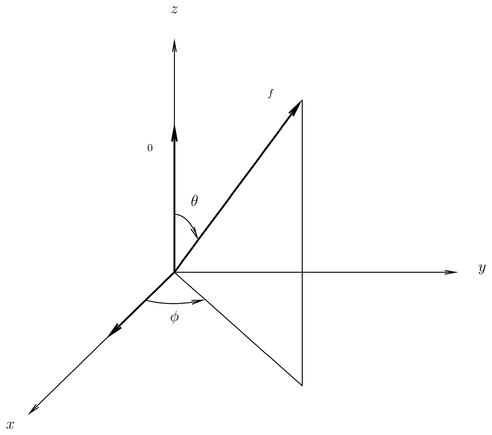
Figure 1:Coordinates for the photoelectric effect.
Angular Dependence and Total Cross Section
We now introduce coordinates, as illustrated in Figure 1. We assume the atom is at the origin, and that the photon comes in along the negative -axis, so that . The photon is assumed to be linearly polarized in the -direction, so that . The ejected electron goes out in the direction .
With the geometry indicated in Figure 1 and the approximations (43) and (45), we can simplify the cross (38). We find
This is the cross for linear polarization in the -direction. If we had had linear polarization in the -direction, we would have obtained in (46) instead of . To deal with the case of unpolarized light, we must average over initial polarizations; this can be carried out formally by using a density matrix for the photons, but in the present case it amounts to adding and and dividing by 2. If we also expand the denominator to first order in , we obtain
Finally, we can integrate this over all solid angles of the final ejected electron, whereupon the term in disappears, to obtain the total cross for unpolarized radiation,
The total cross can be written in various ways; for example, we can express it in terms of the incident photon energy and the Bohr radius of hydrogen:
where is the fine structure constant. In this form the cross is manifestly an area, since is essentially the cross-al area of a hydrogen atom. This area is reduced by the very small factor , but magnified by the presumably large factor (because of the nonrelativistic assumption ), and by the possibly large factor . Although this formula was derived only for a hydrogen-like atom, it is valid in a semiquantitative way for the ejection of -shell electrons by x-rays in any atom. The strong -dependence indicates that heavier atoms are more effective in stopping x-rays, and the strong inverse energy dependence indicates that hard x-rays are more penetrating than soft ones.
Problems
Problem 1.
X-rays of energy that are linearly polarized in the -direction are incident upon positronium in the ground state. The beam of x-rays is directed in the direction. The positronium atom'' is at rest. Find the differential cross section $d\sigma/d\Omega$ for the x-ray to break the atom’’ apart, where refers to the direction of the ejected electron. Assume
where is the usual (hydrogen) Bohr radius, and make approximations this set of notes. In particular, expand your answer through first order in . Find the total cross and express it as a function of , and as a multiple of .
Note that the light wave interacts with both the electron and the positron; therefore you must set up a two-particle Hamiltonian.