09. The Propagator and the Path Integral

Introduction¶

The propagator is basically the $x$ -space matrix element of the time evolution operator $U(t,t_0)$ , which can be used to advance wave functions in time. It is closely related to various Green’s functions for the time-dependent Schr"odinger equation that are useful in time-dependent perturbation theory and in scattering theory. We provide only a bare introduction to the propagator in these notes, just enough to get started with the path integral, which is our main topic. Later when we come to scattering theory we will look at propagators and Green’s functions more systematically.

The path integral is an expression for the propagator in terms of an integral over an infinite-dimensional space of paths in configuration space. It constitutes a formulation of quantum mechanics that is alternative to the usual Schr"odinger equation, which uses the Hamiltonian as the generator of displacements in time. The path integral, on the other hand, is based on Lagrangians. This is particularly useful in relativistic quantum mechanics, where we require equations of motion that are Lorentz covariant. These are achieved by making the Lagrangian a Lorentz scalar, that is, independent of Lorentz frame. In contrast, Hamiltonians are always dependent on the choice of Lorentz frame, since they involve a particular choice of the time parameter. This is one advantage of the path integral over the usual formulation of quantum mechanics in terms of the Schr"odinger equation.

In fact, the path integral or Lagrangian formulation of quantum mechanics involves characteristically different modes of thinking and a different kind of intuition than those useful in the Schr"odinger or Hamiltonian formulation. These alternative points of view are very effective in certain classes of problems, where they lead quickly to some understanding of the physics that would be more difficult to obtain in the Schr"odinger or Hamiltonian formulation.

In addition, path integrals simplify certain theoretical problems, such as the quantization of gauge fields and the development of perturbation expansions in field theory. For these and other reasons, path integrals have assumed a central role in most areas of modern quantum physics, including particle physics, condensed matter physics, and statistical mechanics.

However, for most simple nonrelativistic quantum problems, the path integral is not as easy to use as the Schr"odinger equation, and most of the results obtained with it can be obtained more easily by other means. Nevertheless, the unique perspective afforded by the path integral as well as the many applications to which it can be put make it an important part of the study of the fundamental principles of quantum mechanics.

Standard references on path integrals include the books Quantum Mechanics and Path Integrals by Feynman and Hibbs and Techniques and Applications of Path Integration by L. S. Schulman. The first chapter of Feynman and Hibbs is especially recommended to those who wish to see a beautiful example of Feynman’s physical insight.

The Propagator¶

In this we will denote the Hamiltonian operator when acting on kets by $\Hhat$ , and we will allow it to depend on time. When we wish to denote the Hamiltonian as a differential operator acting on wave functions in the configuration representation, we will write simply $H$ (without the hat), and we will moreover assume a one-dimensional kinetic-plus-potential form,

H= -{\hbar^2 \over 2m} {\partial^2 \over \partial x^2} + V(x,t).

(1)

The relation between the two notations for the Hamiltonian is

\matrixelement{x}{\Hhat}{\psi} = H\braket{x}{\psi} =\Bigl[ -{\hbar^2\over 2m} {\partial^2 \over \partial x^2} + V(x,t)\Bigr] \psi(x,t),

(2)

where $\ket{\psi}$ is any state. [See (79).] This one-dimensional form is sufficient to convey the general idea of the propagator, and generalizations are straightforward for the applications that we shall consider.

The Hamiltonian $\Hhat(t)$ is associated with a time-evolution operator $U(t,t_0)$ , as discussed in 05. Time Evolution in Quantum Mechanics. The properties of this operator that we will need here are the initial conditions $U(t_0,t_0)=1$ [see (2)] and the equation of evolution [a version of the Schr"odinger equation, (13)]. In addition, we note the composition property (4).

The propagator is a function of two space-time points, a “final” position and time $(x,t)$ , and an “initial” position and time $(x_0,t_0)$ . We define the propagator by

K(x,t;x_0,t_0) = \matrixelement{x}{U(t,t_0)}{x_0},

(3)

so that $K$ is just the $x$ -space matrix element of $U(t,t_0)$ between an initial point $x_0$ (on the right) and a final point $x$ (on the left). It is often described in words by saying that $K$ is the amplitude to find the particle at position $x$ at time $t$ , given that it was at position $x_0$ at time $t_0$ .

The propagator is closely related to various time-dependent Green’s functions that we shall consider in more detail when we take up scattering theory (see 37. Green’s Functions in Quantum Mechanics). These Green’s functions are also often called “propagators,” and they are slightly more complicated than the propagator we have introduced here. The simpler version that we have defined here is all we will need to develop the path integral.

The properties of the propagator closely follow the properties of $U(t,t_0)$ . For example, the initial condition $U(t_0,t_0)=1$ implies

K(x,t_0;x_0,t_0) = \braket{x}{x_0} = \delta(x-x_0).

(4)

Likewise, with the help of (13) we can work out an evolution equation for the propagator,

\begin{aligned} &i\hbar\frac{\partial K(x,t;x_0,t_0)}{\partial t} = \matrixelement{x}{i\hbar\frac{\partial U(t,t_0)}{\partial t}}{x_0} =\matrixelement{x}{\Hhat(t) U(t,t_0)}{x_0} \end{aligned}

(5)

\begin{aligned} &\qquad =H(t) \matrixelement{x}{U(t,t_0)}{x_0} =\Bigl[-{\hbar^2\over 2m} {\partial^2 \over \partial x^2} + V(x,t)\Bigr] K(x,t;x_0,t_0), \end{aligned}

(6)

where we use (2).

We see that the propagator is actually a solution of the time-dependent Schr"odinger equation in the variables $(x,t)$ , while the variables $(x_0,t_0)$ play the role of parameters. Any solution of the time-dependent Schr"odinger equation is characterized by its initial conditions, which in the case of the propagator are given by (4). We see that if we have a “wave function” that at the initial time is given by $\psi(x,t_0) = \delta(x-x_0)$ , then at the final time $\psi(x,t) = K(x,t;x_0,t_0)$ . This is a useful way of thinking of the propagator: it is the solution of the time-dependent Schr"odinger equation with $\delta$ -function initial conditions. These initial conditions are rather singular, however, for example, the initial wave function is not normalizable.

Knowledge of the propagator implies knowledge of the general solution of the time-dependent Schr"odinger equation, that is, with any initial conditions. For if we let $\psi(x,t_0)$ be some arbitrary initial conditions, then the final wave function can be written,

\begin{aligned} \psi(x,t) &= \braket{x}{\psi(t)} = \matrixelement{x}{U(t,t_0)}{\psi(t_0)} =\int dx_0 \, \matrixelement{x}{U(t,t_0)}{x_0} \braket{x_0}{\psi(t_0)} \end{aligned}

(7)

\begin{aligned} &=\int dx_0 \, K(x,t;x_0,t_0) \psi(x_0,t_0). \end{aligned}

(8)

We see that the propagator is the kernel of the integral transform that converts an initial wave function into a final one.

(8) has a pictorial interpretation in terms of Huygen’s principle, which says that the final wave field is the superposition of little waves radiated from each point of the source field, weighted by the strength of the source field at that point. In the present case, each point $x_0$ of the source field at time $t_0$ radiates a wave whose value at field point $x$ at time $t$ is $K(x,t;x_0,t_0)$ , multiplied by $\psi(x_0,t_0)$ . The superposition of all the radiated waves (the integral) is the final wave field.

The initial conditions for the propagator are quite singular. The $\delta$ -function means that at time $t_0$ the particle is concentrated in an infinitesimal region of space. By the uncertainty principle, this means that the initial momentum is completely undetermined, and the wave function contains momentum values all the way out to $p= \pm \infty$ . A classical or semiclassical picture of these initial conditions would be that of an ensemble of particles, all at the same position in space, but with various momenta extending out to arbitrarily large values. Thus, when we turn on time, there is a kind of explosion of particles, with those with high momentum covering a large distance even in a short time. This is true regardless of the potential (as long as it is not a hard wall). Similarly, in quantum mechanics, we find that the wave function, that is, the propagator $K(x,t;x_0,t_0)$ , is nonzero everywhere in configuration space even for small positive times.

The Propagator for the Free Particle¶

Let us compute the propagator for the one-dimensional free particle, with Hamiltonian $H=\phat^2/2m$ . We put a hat on the momentum operator, to distinguish it from momentum $c$ -numbers $p$ to appear in a moment. Since the system is time-independent, we set $t_0=0$ and write $U(t)=U(t,0)$ , and we have $U(t) = \exp(-itH/\hbar)$ . Thus,

K(x,x_0,t) = \, \matrixelement{x}{\exp(-it \phat^2/2m\hbar)}{x_0}.

(9)

We insert a momentum resolution of the identity into this to obtain,

K(x,x_0,t) = \int dp \, \matrixelement{x}{\exp(-it \phat^2/2m\hbar)}{p} \braket{p}{x_0}.

(10)

In the first matrix element in the integrand, the operator $\phat$ is acting on an eigenstate $\ket{p}$ of momentum, so $\phat$ can be replaced by $p$ , making $\exp(-it p^2/2m\hbar)$ , which is a $c$ -number that can be taken out of the matrix element. What remains is $\braket{x}{p}$ . This and the second matrix element in the integrand $\braket{p}{x_0}$ are given by the one-dimensional version of (86). Thus we find

K(x,x_0,t) = \int {dp \over 2\pi\hbar} \, \exp\Bigl\{ {i\over \hbar} \Bigl[ p(x-x_0) - {p^2 t \over 2m}\Bigr] \Bigr\}.

(11)

The integral is easily done [see (6)], with the result

K(x,x_0,t) = \sqrt{ \ds {\ds m \over \ds 2\pi i \hbar t}} \, \exp\Bigl[ {i\over \hbar} {m(x-x_0)^2 \over 2t} \Bigr].

(12)

For reference we record also the propagator for the free particle in three dimensions,

K(\xvec,\xvec_0,t) = \Bigl( {m \over 2\pi i \hbar t} \Bigr)^{3/2} \exp\Bigl[ {i\over \hbar} {m(\xvec-\xvec_0)^2 \over 2t} \Bigr],

(13)

an obvious generalization of the one-dimensional case that is just as easy to derive.

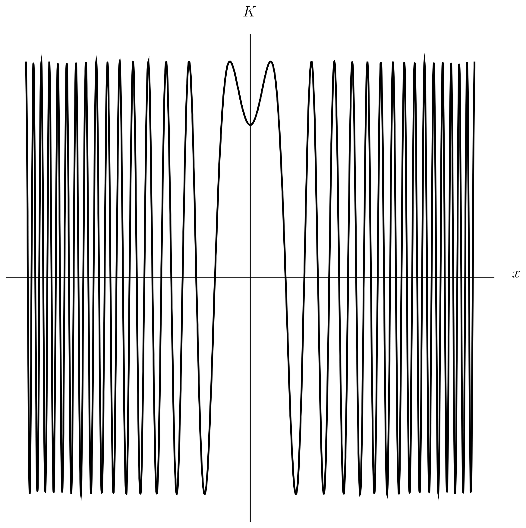
Real part of the free particle propagator at a positive time, with x_0=0. — Figure 1:Real part of the free particle propagator at a positive time, with $x_0=0$ .

Same as , but at a later time. — Figure 2:Same as Figure 1, but at a later time.

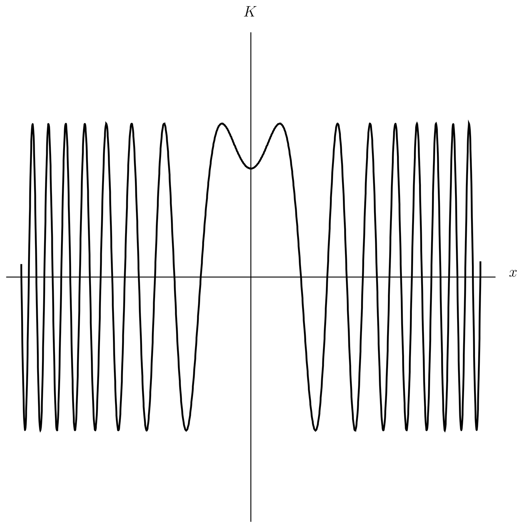
It is of interest to see how the propagator (12) approaches the limit $\delta(x-x_0)$ when $t \to 0^+$ . In view of what we have said above about an explosion of particles, this must be a very singular limit. A plot of the real part of the propagator is shown in Figure 1 at a certain time, and in Figure 2 at a later time. In order to achieve the $\delta$ -function limit, we expect that for fixed $x \ne x_0$ , the propagator should approach zero as $t \to 0^+$ , while precisely at $x=x_0$ it should go to infinity. In fact, what we see from the plot is that at fixed $t$ the propagator is a wave in $x$ of constant amplitude. The amplitude depends only on $t$ , and in fact diverges at all $x$ as $t \to 0^+$ . The wavelength at fixed $t$ depends on $x$ , getting shorter as $x$ increases, and similarly depends on $t$ at fixed $x$ , getting shorter as $t$ decreases toward 0. For $x \ne x_0$ , the propagator does not go to zero numerically as $t \to 0^+$ , in fact its value oscillates between limits that go to infinity. It does, however, approach zero in the distribution sense, that is, if it is integrated against a smooth test function, then the positive contribution of one lobe of the wave nearly cancels the negative contribution of the next lobe. As $t\to 0^+$ , the cancellation gets more and more perfect. It is in this sense that the propagator goes to 0 at fixed $x \ne x_0$ as $t \to 0^+$ . In the immediate neighborhood of $x=x_0$ , the propagator has one positive lobe that is not cancelled by neighboring negative lobes. This positive lobe has a width that goes to zero as $t^{1/2}$ and a height that goes to infinity as $t^{-1/2}$ as $t\to 0^+$ , exactly as we expect of a $\delta$ -function. At fixed $x \ne x_0$ , the wavelength gets shorter as $t \to 0^+$ because for short times it is the high momentum particles that get out first. The wavelength is shorter for larger $|x-x_0|$ at fixed $t$ for the same reason.

The free particle is one of the few examples for which the propagator can be evaluated explicitly. Another is the harmonic oscillator. The latter is an important result, but “ordinary” derivations involve special function tricks or lengthy algebra. Instead, it is more educational to derive the propagator for the harmonic oscillator from the path integral.

The Path Integral in One Dimension¶

We now derive the path integral for a one-dimensional problem with Hamiltonian,

H=T+V = {p^2\over 2m} + V(x).

(14)

The path integral is easily generalized to higher dimensions, and time-dependent potentials present no difficulty. With a little extra effort, magnetic fields can be incorporated. But there is greater difficulty in incorporating operators of a more general functional form, such as those with fourth powers of the momentum.

Since the Hamiltonian (14) is time-independent, we can set $t_0=0$ and $U(t)=U(t,t_0) = \exp(-iHt/\hbar)$ . The propagator now depends on only three parameters $(x,x_0,t)$ , where $t$ is the elapsed time. It is given by

K(x,x_0,t) = \matrixelement{x}{U(t)}{x_0}.

(15)

We consider the final time $t$ fixed and we break the interval $[0,t]$ up into a large number $N$ of small intervals of duration $\epsilon$ ,

\epsilon = {t\over N},

(16)

so that

U(t) = [U(\epsilon)]^N.

(17)

We will think of taking the limit $N \to \infty$ , or $\epsilon \to 0$ , holding the final time $t$ fixed. The time evolution operator for time $\epsilon$ is

U(\epsilon) = e^{-i\epsilon(T+V)/\hbar}.

(18)

Because the kinetic energy $T$ and potential energy $V$ do not commute, the exponential of the sum in (18) is not equal to the product of the exponentials, $e^{-i\epsilon T/\hbar} e^{-i\epsilon V/\hbar}$ . But since $\epsilon$ is small, such a factorization is approximately correct, as we see by expanding in Taylor series:

U(\epsilon) = 1 -{i\epsilon\over\hbar}(T+V) + O(\epsilon^2) =e^{-i\epsilon T/\hbar} \, e^{-i\epsilon V/\hbar} +O(\epsilon^2).

(19)

The term $O(\epsilon^2)$ is also $O(1/N^2)$ , so when we raise both sides of (19) to the $N$ -th power we obtain

U(t) = \bigl[ e^{-i\epsilon T/\hbar} \, e^{-i\epsilon V/\hbar} \bigr]^N + O(1/N).

(20)

This argument is far from rigorous---in fact, it is difficult to treat the Feynman path integral rigorously---but the line of reasoning can be used to obtain correct results and is very useful in physical applications.

Therefore we can write

K(x,x_0,t) = \lim_{N\to\infty} \matrixelement{x} { \bigl[ e^{-i\epsilon T/\hbar} \, e^{-i\epsilon V/\hbar} \bigr]^N }{x_0}.

(21)

There are $N$ factors here, so we can put $N-1$ resolutions of the identity between them. We write the result in the form,

\begin{aligned} & K(x,x_0,t) = \lim_{N\to\infty} \int dx_1 \, \ldots \, dx_{N-1} \end{aligned}

(22)

\begin{aligned} &\quad \times \matrixelement{x_N}{ e^{-i\epsilon T/\hbar} \, e^{-i\epsilon V/\hbar} }{x_{N-1}} \matrixelement{x_{N-1}}{\, \ldots \,}{x_1} \matrixelement{x_1}{e^{-i\epsilon T/\hbar} \, e^{-i\epsilon V/\hbar}}{x_0}, \end{aligned}

(23)

where we have set

x=x_N,

(24)

in order to achieve greater symmetry in the use of subscripts.

Let us evaluate one of the matrix elements appearing in (23), the one involving the bra $\bra{x_{j+1}}$ and the ket $\ket{x_j}$ . By inserting a resolution of the identity in momentum space, we have

\matrixelement {x_{j+1}} {e^{-i\epsilon T/\hbar}\, e^{-i\epsilon V/\hbar}}{x_j} = \int dp\, \matrixelement{x_{j+1}} {e^{-i\epsilon\phat^2/2m\hbar}}{p} \matrixelement{p}{e^{-i\epsilon V(\xhat)/\hbar}} {x_j},

(25)

where $\xhat$ and $\phat$ are operators. These however act on eigenstates of themselves, giving the integral,

\int {dp\over 2\pi\hbar}\, \exp\Bigl\{{i\over\hbar}\Bigl[ -\epsilon{p^2\over 2m} +p(x_{j+1}-x_j) -\epsilon V(x_j)\Bigr]\Bigr\},

(26)

which is almost the same as the integral (11). The result is

\matrixelement {x_{j+1}} {e^{-i\epsilon T/\hbar}\, e^{-i\epsilon V/\hbar}}{x_j} = \sqrt{\ds{\ds m\over \ds 2\pi i \epsilon\hbar}}\, \exp\Bigl\{ {i\over\hbar}\Bigl[ m{(x_{j+1}-x_{j})^2 \over 2\epsilon} -\epsilon V(x_j)\Bigr]\Bigr\}.

(27)

When this is inserted back into (23), we obtain a product of exponentials that can be written as the exponential of a sum. The result is

\begin{aligned} &K(x_0,x,t) = \lim_{N\to\infty} \left( {m\over 2\pi i\hbar\epsilon} \right)^{N/2} \int dx_1 \ldots dx_{N-1} \end{aligned}

(28)

\begin{aligned} &\qquad \times \exp \Bigl\{ {i\epsilon\over\hbar} \sum_{j=0}^{N-1} \Bigl[ {m(x_{j+1} - x_j)^2 \over 2\epsilon^2} -V(x_j) \Bigr] \Bigr\}. \end{aligned}

(29)

This is a discretized version of the path integral in configuration space.

Visualization, and Integration in Path Space¶

To visualize the integrations being performed in this integral, we observe that $x_0$ and $x_N=x$ are fixed parameters of the integral, being the $x$ -values upon which $K$ depends, whereas all the other $x$ ’s, $x_1$ , $\ldots$ , $x_{N-1}$ , are variables of integration. Therefore we identify the sequence of numbers, $(x_0,x_1, \ldots, x_N)$ with a discretized version of a path $x(t)$ in configuration space with fixed endpoints $(x_0,x_N=x)$ , but with all intermediate points being variables. We think of the path $x(t)$ as passing through the point $x_j$ at time $t_j = j\epsilon$ , so that $t_0=0$ and $t_N=t$ . See Figure 3, in which the heavy line is the discretized path, with fixed endpoints $(x_0,t_0)=(x_0,0)$ and $(x,t)=(x_N,t_N)$ . The intermediate $x_i$ , $i=1, \ldots, N-1$ are variables of integration that take on all values from $-\infty$ to $+\infty$ , each effectively running up and down one of the dotted lines in the figure. Then as $N\to\infty$ , we obtain a representation of the path at all values of $t$ , and the integral turns into an integral over an infinite space of paths $x(t)$ in configuration space, which are constrained to satisfy given endpoints at given endtimes.

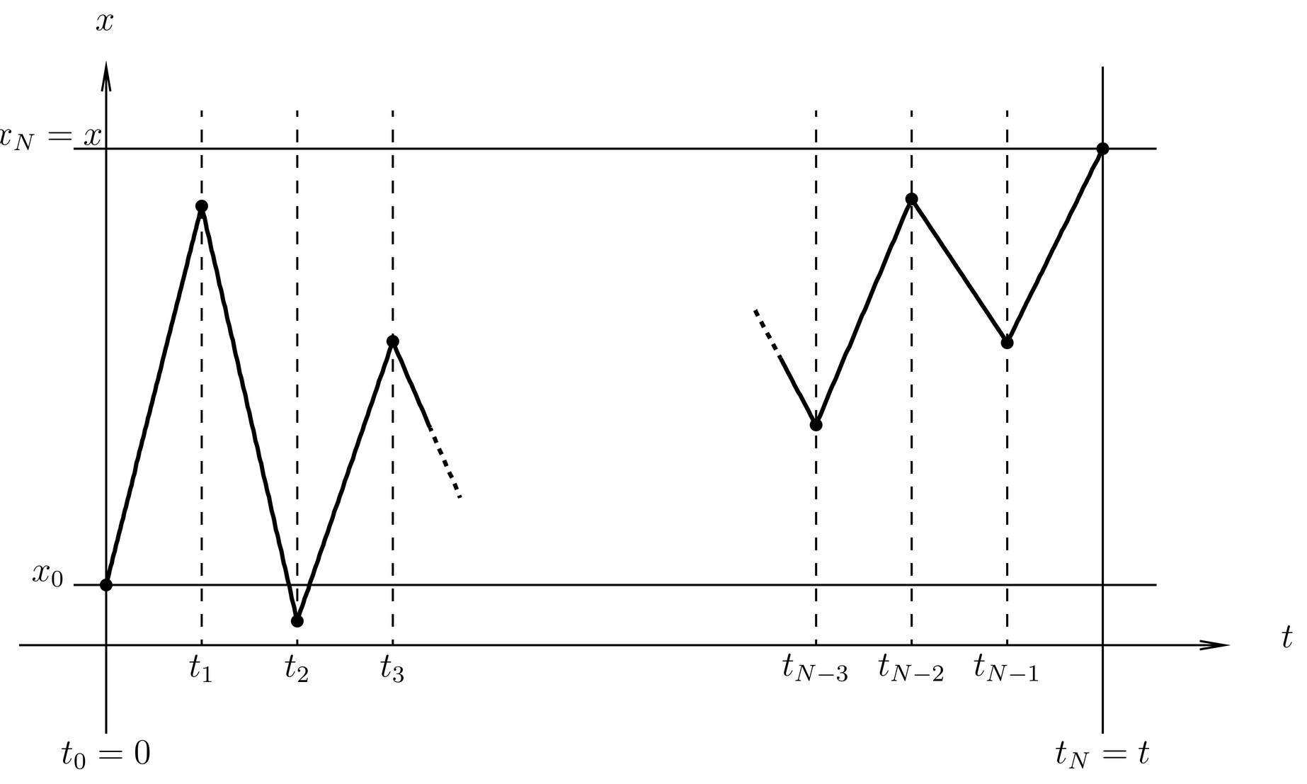
A space-time diagram to visualize the integrations in the discretized version of the path integral in configuration space, Eq. . — Figure 3:A space-time diagram to visualize the integrations in the discretized version of the path integral in configuration space, Eq. (29).

Notice that if we set $\Delta t=\epsilon$ and $\Delta x_j = x_{j+1}-x_j$ , then the exponent in (29) looks like $i/\hbar$ times a Riemann sum,

\Delta t \sum_{j=0}^{N-1} \Bigl[{m\over 2} \Bigl( {\Delta x_j \over \Delta t}\Bigr)^2 - V(x_j)\Bigr],

(30)

which is apparently an approximation to the integral,

A[x(\tau)] = \int_0^t d\tau \, \Bigl[{m\over 2} \Bigl( \dod{x}{\tau}\Bigr)^2 -V(x)\Bigr] = \int_0^t d\tau \, L\bigl(x(\tau),{\dot x}(\tau)\bigr),

(31)

where $L$ is the classical Lagrangian,

L(x,\dot x) = {m\dot x^2\over 2} - V(x).

(32)

The quantity $A[x(\tau)]$ is the “action” of the path $x(\tau)$ , $0\le \tau \le t$ , that is, the integral of the Lagrangian along the path. In fact, the Riemann sum (30) would approach the integral (31) as $N\to\infty$ if the path $x(\tau)$ were sufficiently well behaved (this is the definition of the integral), but, as we shall see, the paths involved are usually not well behaved. Nevertheless, these considerations motivate a more compact notation for the path integral,

K(x,x_0,t) = C \int d[x(\tau)] \, \exp \Bigl( {i\over\hbar} \int_0^t L \, d\tau \Bigr),

(33)

where $C$ is the normalization constant seen explicitly in the discretized form (29), and where $d[x(\tau)]$ represents the “volume” element in the infinite-dimensional path space. The compact form (33) of the path integral is easier to remember or write down than the discretized version (29), and easier to play with, too.

Remarks on the Path Integral¶

As we have remarked, the path integral constitutes a complete formulation of quantum mechanics that is alternative to the usual one, based on the Schr"odinger equation and Hamiltonians. Certainly the path integral is especially well adapted to time-dependent problems because it is an expression for the propagator. But if we want energy eigenvalues and eigenfunctions (the usual goal of the Schr"odinger-Hamiltonian approach), those can also be obtained by Fourier transforming in time any solution $\psi(x,t)$ of the time-dependent Schr"odinger equation, including the propagator $K(x,x_0,t)$ itself. Anything that can be done with the Schr"odinger-Hamiltonian approach to quantum mechanics can in principle also be done with the path integral, and vice versa. Moreover, both provide routes for quantization, that is, passing from classical mechanics to quantum mechanics, one of which uses the Hamiltonian, the other the Lagrangian.

But we may ask which approach is more fundamental. Not to get into philosophical debates, but there are indications that the path integral or Lagrangian approach is more fundamental. It is the classical Lagrangian that appears in the path integral, that is, the exponent is just a number, the integral of the Lagrangian along a path (there is no “Lagrangian operator”). This has definite advantages in relativistic quantum mechanics, as already pointed out, that is, to guarantee Lorentz covariance of the results we need only use a Lagrangian that is a Lorentz scalar. Feynman made good use of this feature in the early history of path integrals to develop covariant approaches to quantum electrodynamics. (See the reprint, “I can do that for you!” for Feynman’s recollections of that period.)

In addition, you may note the simple manner in which $\hbar$ appears in (33). It is just the unit of action, which serves to make the exponent dimensionless. You may compare this to the more complicated and less transparent manner in which $\hbar$ appears in the Schr"odinger equation.

The propagator $K(x,x_0,t)$ is the amplitude to find the particle at position $x$ at time $t$ , given that it was at position $x_0$ at time $t_0=0$ . We may be tempted to ask where the particle was at intermediate times, but we must be careful with the concepts implied by such a question because we cannot measure the particle at an intermediate time without altering the wave function and hence the amplitude to find the particle at position $x$ at the final time. This is like the double slit experiment, in which a beam passes through two slits and forms an interference pattern on a screen. Did the particle somehow go through both slits at the same time? If we try to observe which slit the particle went through, by shining light just beyond the slit openings and looking for scattered photons, we will find that any individual particle only goes through one slit. But the act of measuring the particle changes the wave function, and the interference pattern disappears.

The interference pattern is the square of the sum of two amplitudes, that is, the two wave functions emanating from the two slits. This is a general rule in quantum mechanics, that the amplitude for a collection of intermediate possibilities is the sum of the amplitudes over those possibilities, and the probability is the square of the amplitude. This is an interpretation of the insertion of a resolution of the identity into an amplitude, one is summing over all amplitudes corresponding to intermediate possibilities.

In the case of the path integral, the amplitude to find the particle at the final position $x$ at time $t$ , given that it was at $x_0$ at time $t_0=0$ , is a sum (the path integral) of amplitudes corresponding to all intermediate possibilities, that is, all paths connecting the two endpoints. The amplitude for each of these paths (the integrand in the path integral) is a constant times a phase factor, $\exp\{(i/\hbar)A[x(t)]\}$ . The square of the phase factor is just 1, so we can say that all paths connecting the initial and final points in the given amount of time are equally probable, including paths that are completely crazy from a classical standpoint. In this sense, there is complete democracy among all the paths that enter into the path integral. This is true regardless of the potential.

Of course, the potential does make a difference. It does so by changing the phases of the amplitudes associated with each path, which changes the patterns of constructive and destructive interference among the amplitudes of the different paths. Remember that in quantum mechanics, amplitudes add, and probabilities are the squares of amplitudes. All of the physics that we associate with a given potential is the result of the interference of these amplitudes.

The Nature of the Paths in the Path Integral¶

Since only the endpoints $x_0$ and $x_N=x$ are fixed in the path integral (29), and since all intermediate points are variables of integration, it is clear that the paths that contribute to the path integral include some that are very strange looking. To visualize this, let us take the discretized version of the path integral and hold all the variables of integration fixed except one, say, $x_j$ . If we write $\Delta x = x_j - x_{j-1}$ , then during the integration over $x_j$ , $\Delta x$ takes on all values from $-\infty$ to $+\infty$ . This is true regardless of how small $\epsilon = \Delta t$ gets. This suggests that most of the paths $x(t)$ that go into the path integral are not even continuous, since in time interval $\Delta t = \epsilon$ any arbitrarily large value of $\Delta x$ is allowed. But this conclusion is too drastic, and in a sense is not really correct. For as we will see later, it is appropriate to regard only those paths for which $\Delta x \sim \sqrt{\Delta t}$ as contributing to the path integral, in spite of the fact that the absolute value of the integrand (namely unity) does not go to zero as $\Delta x$ gets large. (Instead, this integrand oscillates itself to death as $\Delta x$ gets large). In this interpretation, we see that the paths that contribute to the path integral are indeed continuous, for if $\Delta x \sim \sqrt{\Delta t}$ , then as $\Delta t\to0$ , we also have $\Delta x \to 0$ . On the other hand, most of these paths are not differentiable, for we have $\Delta x/\Delta t \sim (\Delta t)^{-1/2}$ as $\Delta t \to 0$ . Thus, a typical path contributing to the path integral is continuous everywhere but differentiable nowhere, and in fact has infinite velocity almost everywhere. To visualize such paths you may think of white noise on an oscilloscope trace, or a random walk such as Brownian motion in the limit in which the step size goes to zero. As you no doubt know, random walks also lead to the rule $\Delta x \sim \sqrt{\Delta t}$ . Indeed path integrals of a different form (the so-called Wiener integral, with real, damped exponents instead of oscillating exponentials) are important in the theory of Brownian motion and similar statistical processes.

If typical paths in the path integral are not differentiable, that is, if in some sense they have infinite velocity everywhere, then what is the meaning of the kinetic energy term in the Lagrangian in (30)? In fact, there is indeed an interpretational problem in the evaluation the action integral for such paths, and for this reason the compact notation (33) for the path integral glosses over some things that are dealt with more properly in the discretized version (29). In physical applications this discretized version is meaningful and the limit can be taken; one must resort to this procedure when questions concerning the differentiability of paths arise. Furthermore, the discretized version of the action integral in (29) is not really a Riemann sum approximation to a classical action integral, because in classical mechanics we (almost) always deal with paths that are differentiable. Instead, the integral is of a different type (an Ito integral). Nevertheless, in many applications we can use the rules of ordinary calculus (that is, Riemann integrals) when manipulating the action integral in the exponent of the path integral. Some of these will be explored in the problems.

Stationary Action and Hamilton’s Principle¶

The action integral (31) that appears in the exponent of the path integral (33) is suggestive of classical mechanics (see Appendix~\classmech), where it is shown that the paths that are the solutions of Newton’s equations cause the action to be stationary. These classical paths are usually smooth, so the action integral in classical mechanics is an ordinary Riemann integral.

The question then arises, how do these classical paths make their privileged status known in the limit in which $\hbar$ is small compared to typical actions of the problem? That is, how does the classical limit appear in the path integral formulation of quantum mechanics?

The answer lies in the principle of stationary phase, which says that in an integral with a rapidly oscillating integrand, the principal contributions come from regions of the variable of integration that surround points where the phase is stationary, that is, where it has only second order variations under first order variations in the variable of integration. This is because the integrand is in phase with itself in the neighborhood of stationary phase points, and so interferes constructively with itself. In the path integral, the variable of integration is a path and the phase is the action along that path, so the stationary phase “points” are the paths of path

space that satisfy {\delta A \over \delta x(t)} =0. This equation is often written in a slightly

(34)

different form, \delta \int L\,dt=0. But this

(35)

is precisely the condition that $x(t)$ should be a classical path, according to Hamilton’s principle in classical mechanics.

This is a remarkable and astonishing result. The variational formulation of classical mechanics, which was fully developed almost a hundred years before quantum mechanics, is based on the observation that the solutions of the classical equations of motion cause a certain quantity, the action defined by (31), to be stationary under small variations in the path. This is something that can be checked by comparing the results with Newton’s laws, and it works in the case that the force is derivable from a potential. It works in some other cases, too, such as magnetic forces, which however require a modified Lagrangian. But why it should work, that is, why nature should endow the classical equations of motion with a variational structure, was a complete mystery until the path integral came along.

The Variational Formulation of Classical Mechanics¶

We will now review the variational formulation of classical mechanics, which is usually taught in at least sketchy form in undergraduate courses in classical mechanics, emphasizing the features that will be important for application to path integrals. See Appendix~\classmech{} for more on classical mechanics.

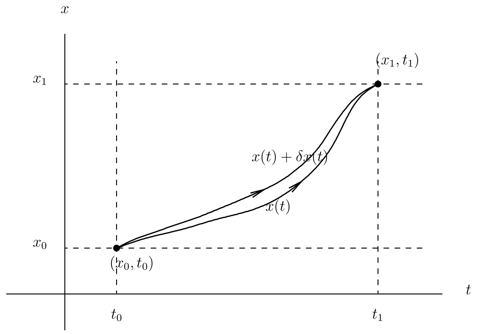
A space-time diagram showing a path x(t) and a modified path x(t)+\delta x(t), both passing through the given endpoints and endtimes (x_0,t_0), (x_1,t_1). — Figure 4:A space-time diagram showing a path $x(t)$ and a modified path $x(t)+\delta x(t)$ , both passing through the given endpoints and endtimes $(x_0,t_0)$ , $(x_1,t_1)$ .

We work with a one-dimensional problem with the Lagrangian $L(x,\xdot) = m\xdot^2/2-V(x)$ . We choose initial and final times $t_0$ and $t_1$ , and initial and final positions, $x_0$ and $x_1$ , which together define a rectangle in a space-time diagram as illustrated in Figure 4. The initial space-time point $(x_0,t_0)$ is at the lower left corner of the rectangle, while the final point $(x_1,t_1)$ is at the upper right.

For the purposes of this classical problem we define a “path” as a smooth function $x(t)$ such that $x(t_0)=x_0$ and $x(t_1)=x_1$ , that is, the path must pass through the given endpoints at the given endtimes. The path need not be a physical path, that is, a solution to Newton’s equations of motion.

Next, we define the “action” of the path as the integral of the Lagrangian along the path, that is,

A[x(t)] = \int_{t_0}^{t_1} L\bigl(x(t),\xdot(t)\bigr) \, dt = \int_{t_0}^{t_1} \Bigl[ {m\over 2}\xdot(t)^2 - V\bigl(x(t)\bigr)\Bigr]\,dt,

(36)

where we have used the explicit form of the Lagrangian. The action is a functional of the path, and is defined for any smooth path, physical or nonphysical. Then Hamilton’s principle asserts that a path is physical, that is, a solution of Newton’s equations of motion, if and only if (34) holds. We can put this into words by saying that first order variations about a physical path cause only second order variations in the action.

You may not be familiar with the functional derivative notation used in (34), but the following will explain the idea. Let $x(t)$ be any path satisfying the endpoint and endtime conditions, as in Figure 4, and let $x(t)+\delta x(t)$ be a nearby path that also satisfies the endpoint and endtime conditions, as in the figure. The notation $\delta x(t)$ indicates the difference between the two paths; thus, $\delta x(t)$ is just a function of $t$ , and the $\delta$ that appears here is not an operator. It is, however, a reminder that the function $\delta x(t)$ is small. Since both paths $x(t)$ and $x(t)+\delta x(t)$ satisfy the endpoint and endtime conditions, we have

\delta x(t_0) = \delta x(t_1) = 0.

(37)

Now we evaluate the action along the modified path, obtaining

\begin{aligned} A[x(t)+\delta x(t)] &= \int_{t_0}^{t_1} \Bigl\{ {m\over 2} \bigl[ \xdot(t) + \delta \xdot(t)\bigr]^2 - V\bigl( x(t) + \delta x(t)\bigr)\Bigr\} \, dt \\ &=\int_{t_0}^{t_1} \Bigl\{ {m\over 2}\bigl[ \xdot(t)^2 + 2 \xdot(t)\, \delta \xdot(t) + \delta \xdot(t)^2 \bigr] \\ &\quad - V\bigl(x(t)\bigr) - V'\bigl(x(t)\bigr)\, \delta x(t) -{1\over 2}V''\bigl(x(t)\bigr) \,\delta x(t)^2 - \ldots \Bigr\} \, dt \\ &=T_0 + T_1 + T_2 + \ldots, \\ \end{aligned}

(38)

where we have expanded the integrand in powers of $\delta x(t)$ and written the zeroth order, first order, etc.{} terms as $T_0$ , $T_1$ , etc. The zeroth order term is just the action evaluated along the unmodified path $x(t)$ ,

T_0 = \int_{t_0}^{t_1} \Bigl[ {m\over 2}\xdot(t)^2 - V\bigl( x(t) \bigr)\Bigr]\, dt = A[x(t)].

(39)

The first order contribution to the action, $T_1$ , has two terms, of which we integrate the first by parts to obtain

\begin{aligned} T_1 &= \int_{t_0}^{t_1} \Bigl[ m\xdot(t)\,\delta\xdot(t) -V'\bigl(x(t)\bigr)\,\delta x(t)\Bigr]\, dt \\ &= \Bigl. m \xdot(t)\,\delta x(t)\Bigr|_{t_0}^{t_1} + \int_{t_0}^{t_1} \Bigl[ -m{\ddot x}(t)\,\delta x(t) -V'\bigl(x(t)\bigr)\,\delta x(t)\Bigr]\, dt. \\ \end{aligned}

(40)

The boundary term vanishes because of (37), and the rest can be written,

T_1 = \int_{t_0}^{t_1} \Bigl[ -m{\ddot x}(t) -V'\bigl( x(t)\bigr)\Bigr]\,\delta x(t)\, dt.

(41)

We see that $T_1$ vanishes if the path $x(t)$ is physical, that is, if it satisfies Newton’s laws,

m\ddot x = -V'(x).

(42)

Conversely, if $T_1=0$ for all choices of $\delta x(t)$ , then the Newton’s laws (42) must be satisfied. This is Hamilton’s principle for the type of one-dimensional Lagrangian we are considering. The notation in (34) in the present case is

{\delta A \over \delta x(t)} = -m{\ddot x}(t) -V'\bigl( x(t)\bigr),

(43)

that is, the functional derivative shown is just the integrand of (41) with the $\delta x(t)$ stripped off.

Is the Action Really Minimum? (or Extremum?)¶

Books on classical mechanics often say that the classical paths minimize the action, and Sakurai Modern Quantum Mechanics repeats this misconception. Other books say that it is an extremum (a maximum or minimum). In fact, the action is sometimes a minimum along the classical path, and other times not. It is correct to say that the classical path causes the action to be stationary, that is, the first order variations in the action about a classical path vanish. Insofar as classical mechanics is concerned, it does not matter whether the action is minimum, maximum, or just stationary, since the main object of the classical variational principle is the equations of motion. But in applications to the path integral, it does matter, as we shall see.

To see whether the action is minimum or something else along a classical path, we must look at the second order term $T_2$ in (38). Here we are assuming that $x(t)$ is a classical path so $T_1=0$ and $T_2$ is the first nonzero correction to the action along the classical path. This term is

\begin{aligned} T_2 &= \int_{t_0}^{t_1} \Bigl[ {m\over 2} \delta\xdot(t)^2 - {1\over 2} V''\bigl(x(t)\bigr) \, \delta x(t)^2 \Bigr] dt \\ &= \int_{t_0}^{t_1} \Bigl[ -{m\over 2} \delta{\ddot x}(t)\, \delta x(t) - {1\over 2} V''\bigl(x(t)\bigr) \, \delta x(t)^2\Bigr]dt, \\ \end{aligned}

(44)

where we have integrated the first term by parts and dropped the boundary term, as we did with $T_1$ . If $T_2$ is positive for all choices of $\delta x(t)$ , then the action is truly a minimum on the classical path, since small variations about the classical path can only increase the action.

To put this question into a convenient form, let $f(t)$ , $g(t)$ etc be real functions defined on $t_0\le t\le t_1$ that vanish at the endpoints, $f(t_0) = f(t_1) =0$ , etc. Also, define a scalar product of $f$ and $g$ in a Dirac-like notation by

\braket{f}{g} = \int_{t_0}^{t_1} f(t)g(t) \, dt.

(45)

These functions form a Hilbert space, and the scalar product looks like that of wave functions $\psi(x)$ in quantum mechanics except the variable of integration is $t$ instead of $x$ . The boundary conditions are like those of a particle in a box. The only reason we do not put a $*$ on $f(t)$ in (45) is that $f(t)$ is real. Now let us write (44) in the form,

T_2 = \int_{t_0}^{t_1} \delta x(t) \Bigl[ -{m\over2} {d^2 \over dt^2} - {1\over 2} V''\bigl(x(t)\bigr)\Bigr] \delta x(t) \, dt.

(46)

This leads us to define an operator,

B = -{m\over2} {d^2 \over dt^2} - {1\over 2} V''\bigl(x(t)\bigr),

(47)

which acts on functions of $t$ . Remember, $x(t)$ here is just a given function of $t$ (some classical path connecting the given endpoints at the given endtimes). Then the second order variation in the action can be written in a suggestive notation,

T_2 = \matrixelement{\delta x}{B}{\delta x}.

(48)

Thus the condition that $T_2>0$ for all nonzero variations $\delta x(t)$ is equivalent to the statement that $B$ is positive definite, which in turn means that all of its eigenvalues are positive. If, on the other hand, $B$ has some negative eigenvalues, then there are variations $\delta x(t)$ (the eigenfunctions of $B$ corresponding to the negative eigenvalues) which cause the action to decrease about the value along the classical path. In this case the action is not minimum along the classical path.

Uniqueness of the Classical Paths¶

Another misconception about the variational formulation of classical mechanics, also repeated in many books, is that given the endpoints and endtimes, $(x_0,t_0)$ and $(x_1,t_1)$ , there is a unique classical path connecting them. That this is not so is easily seen by the example of a particle in the box, as illustrated in Figure 5. The particle is confined by walls at $x=0$ and $x=L$ . Let the particle be at $x_0=0$ at initial time $t=0$ , and let it be once again at $x_1=0$ at final time $t_1=T$ , where $T>0$ . Then one classical orbit that connects the given endpoints and endtimes is $x(t)=0$ for all $t$ , the orbit that goes nowhere. Another is one that starts with an initial velocity $\xdot(0)=2L/T$ , which causes the particle to bounce once off the wall at $x=L$ and return to $x=0$ at time $T$ . Yet another has initial velocity $4L/T$ , which bounces three times before returning, etc. In this example there are an infinite number of classical orbits satisfying the given boundary conditions.

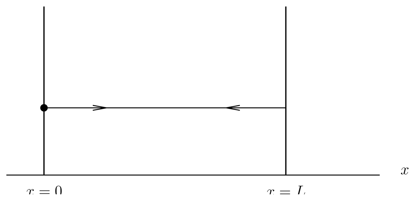
A particle in a box. There are an infinite number of classical orbits connecting x=0 with x=0 in a given amount of time T. — Figure 5:A particle in a box. There are an infinite number of classical orbits connecting $x=0$ with $x=0$ in a given amount of time $T$ .

This example illustrates the fact that the classical orbits satisfying given endpoints and endtimes generally form a discrete set. We will label the orbits by a “branch index”, $b=1,2,\ldots$ . The number of allowed classical orbits (depending on the system and the endpoints and endtimes) can range from zero (in which no classical orbit exists satisfying the given boundary conditions) to infinity (as with the particle in the box).

Hamilton’s Principal Function¶

As noted, the zeroth order term $T_0$ in (38) or (39) is just the action along the original, unmodified path $x(t)$ . It is defined for all paths satisfying the endpoint and endtime conditions, not just physical paths. But if $x(t)$ is a physical path, that is, a solution of Newton’s equations, is there anything special about the value of the action? Hamilton asked himself this question, and found that this is indeed an interesting quantity. The physical path is parameterized by the endpoints and endtimes, as well as by the branch index $b$ , so we define

S_b(x_0,t_0,x_1,t_1) = A[x_b(t)],

(49)

where $x_b(t)$ is the $b$ -th path that satisfies Newton’s equations as well as the boundary conditions. Notice that $S_b$ is an ordinary function of the endpoints and endtimes, unlike $A$ which is a functional (something that depends on a function, namely, the path $x(t)$ ). Confusingly, both $A$ and $S$ are called “the action” (and of course they both have dimensions of action), so you must be careful to understand which is meant when this terminology is used. The function $S_b$ is called Hamilton’s principal function.

Hamilton investigated the properties of this function, and found that it is the key to a powerful method for solving problems in classical mechanics. He showed that this function satisfies a set of differential relations,

\begin{aligned} \frac{\partial S}{\partial x_1} &=p_1, \qquad \frac{\partial S}{\partial t_1}=-H_1, \end{aligned}

(50)

\begin{aligned} \frac{\partial S}{\partial x_0} &=-p_0, \qquad \frac{\partial S}{\partial t_0}=H_0, \end{aligned}

(51)

where $p_0$ , $p_1$ and $H_0$ , $H_1$ are respectively the momentum and Hamiltonian at the two endpoints. Here we have dropped the $b$ index, but these relations apply to each path that satisfies the given boundary conditions. These relations are derived in Hamilton’s Principal Function.

In the special case that the Lagrangian is time-independent, then energy is conserved, $H_0=H_1$ , and $S$ is a function only of the elapsed time $t_1-t_0$ . In this case we often set $t_0=0$ and write simply $S(x_1,x_0,t_1)$ .

The Stationary Phase Approximation¶

We will now explain an approximation for integrals with rapidly oscillating integrands that allows us to connect the path integral (29) with Hamilton’s principle in classical mechanics, and at the same time gives us an approximation for the path integral itself. Roughly speaking, we can think of the integrand of (29) as rapidly oscillating if $\hbar$ (which appears in the denominator of the exponent) is small. Of course, small $\hbar$ corresponds to the classical limit. The approximation is called the stationary phase approximation.

We begin with a 1-dimensional integral of the form,

\int dx\, e^{i\varphi(x)/\kappa},

(52)

where $\kappa$ is a parameter. We wish to examine the behavior of this integral when $\kappa$ is small. Under these circumstances, the phase is rapidly varying, that is, it takes only a small change $\Delta x$ (of order $\kappa$ ) to bring about a change of $2\pi$ in the overall phase. Therefore the rapid oscillations in the integrand nearly cancel one another, and the result is small. But an exception occurs around points $\bar x$ at which the phase is stationary, that is, points $\bar x$ that are roots of

\dod{\varphi}{x}(\bar x) = 0.

(53)

We will call such a point $\bar x$ a stationary phase point; in mathematical terminology, it is a critical point of the function $\varphi$ . In the neighborhood of a stationary phase point the integrand is in phase for a larger $x$ -interval (of order $\Delta x \sim \kappa^{1/2}$ ) than elsewhere, and furthermore there is one lobe of the oscillating integrand that is not cancelled by its neighbors. Therefore we obtain a good approximation if we expand the phase about the stationary phase point,

\varphi(x) = \varphi(\bar x) + y \varphi'(\bar x) + {y^2\over 2} \varphi''(\bar x) + \ldots,

(54)

where $y=x-\bar x$ and where the linear correction term on the right hand side vanishes because of (53). Retaining terms through quadratic order and substituting this into (52), we obtain a Gaussian integral with purely imaginary exponent. This can be done (see Appendix~\gaussint),

\int dx\, e^{i\varphi(x)/\kappa} \approx e^{i\varphi(\bar x)/\kappa} \int dy \, e^{iy^2\varphi''(\bar x)/2\kappa}= \sqrt{ \displaystyle {\displaystyle 2\pi i\kappa \over \displaystyle \varphi''(\bar x)}} \, e^{i\varphi(\bar x)/\kappa}.

(55)

This result is valid if $\varphi''(\bar x)$ is not too small. If $\varphi''(\bar x)$ is very small or if it vanishes, then one must go to cubic order in the expansion (54) (a possibility we will not worry about).

The square root in (55) involves complex numbers, and the notation does not make the phase of the answer totally clear. The following notation is better:

\int dx\, e^{i\varphi(x)/\kappa} = e^{i\nu\pi/4} \sqrt{ \displaystyle {\displaystyle 2\pi \kappa \over \displaystyle |\varphi''(\bar x)| }} \, e^{i\varphi(\bar x)/\kappa},

(56)

where

\nu = \sgn \varphi''(\bar x).

(57)

See (2). Finally, we must acknowledge the possibility that there might be more than one stationary phase point (the roots of (53), which in general is a nonlinear equation). Indexing these roots by a branch index $b$ , the final answer is then a sum over branches,

\int dx\, e^{i\varphi(x)/\kappa} = \sum_b e^{i\nu_b\pi/4} \sqrt{ \displaystyle {\displaystyle 2\pi \kappa \over \displaystyle |\varphi''(\bar x_b)| }} \, e^{i\varphi(\bar x_b)/\kappa}.

(58)

This is the stationary phase approximation for one-dimensional integrals.

Let us generalize this to multidimensional integrals. For this case we write

x = (x_1, \ldots, x_n),

(59)

without using vector (bold face) notation for the multidimensional variable $x$ . We consider the integral,

\int d^n x\, e^{i\varphi(x)/\kappa}.

(60)

As before, we define the stationary phase points $\bar x$ as the roots of

\frac{\partial \varphi}{\partial x_i} (\bar x) =0, \qquad i=1,\ldots,n,

(61)

that is, places where the gradient of $\varphi$ vanish (again, these are the critical points of $\varphi$ ). Then we expand $\varphi$ to quadratic order about a stationary phase point,

\varphi(x) = \varphi(\bar x) + {1\over2} \sum_{k\ell} y_k y_\ell {\partial^2 \varphi(\bar x) \over \partial x_k \partial x_\ell},

(62)

where we drop the vanishing linear terms and where $y=x-\bar x$ . Then the integral (60) becomes a multidimensional imaginary Gaussian integral,

\int d^n x\, e^{i\varphi(x)/\kappa} = e^{i\varphi(\bar x)/\kappa} \int d^n y\, \exp\Bigl( {i \over 2\kappa} \sum_{k\ell} y_k y_\ell {\partial^2 \varphi(\bar x) \over \partial x_k \partial x_\ell} \Bigr).

(63)

We do this by performing an orthogonal transformation $z = Ry$ , where $R$ is an orthogonal matrix that diagonalizes $\partial^2 \varphi/\partial x_k \partial x_\ell$ . Since $\det R=1$ , we have $d^n y = d^n z$ . Then the integral becomes

\int d^n x\, e^{i\varphi(x)/\kappa} = e^{i\varphi(\bar x)/\kappa} \int d^n z\, \exp\Bigl( {i \over 2\kappa} \sum_{k} \lambda_k z_k^2 \Bigr),

(64)

where $\lambda_k$ are the eigenvalues of $\partial^2\varphi/\partial x_k \partial x_\ell$ . This is a product of 1-dimensional Gaussian integrals that can be done as in (55). The result is

\int d^n x\, e^{i\varphi(x)/\kappa} = e^{i\nu\pi/4} \, (2\pi\kappa)^{n/2} \left| \det {\partial^2 \varphi(\bar x) \over \partial x_k \partial x_\ell} \right|^{-1/2} e^{i\varphi(\bar x)/\kappa},

(65)

where

\nu = \nu_+ - \nu_-,

(66)

where $\nu_\pm$ is the number of ± eigenvalues of $\partial^2 \varphi /\partial x_k \partial x_\ell$ . Finally, if there is more than one stationary phase point, we sum over them to obtain

\int d^n x\, e^{i\varphi(x)/\kappa} = \sum_b e^{i\nu_b\pi/4} \, (2\pi\kappa)^{n/2} \left| \det {\partial^2 \varphi(\bar x_b) \over \partial x_k \partial x_\ell} \right|^{-1/2} e^{i\varphi(\bar x_b)/\kappa}.

(67)

This is the stationary phase approximation for multidimensional integrals.

The Stationary Phase Approximation Applied to the Path Integral¶

Now we return to the discretized version of the path integral, (29), and perform the stationary phase approximation on it. In comparison with the mathematical notes in The Stationary Phase Approximation, we set $\kappa=\hbar$ because we are interested in the classical limit in which $\hbar$ is small. Then the quantity $\varphi$ of The Stationary Phase Approximation becomes the discretized version of the action integral,

\varphi(x_0,x_1,\ldots,x_N) = \epsilon \sum_{j=0}^{N-1} \Bigl[ {m\over2} {(x_{j+1} - x_j)^2\over \epsilon^2} -V(x_j) \Bigr].

(68)

We remember that in the path integral, the initial and final points $x_0$ and $x_N=x$ are fixed parameters, and $(x_1,\ldots,x_{N-1})$ are the variables of integration. We differentiate $\varphi$ twice, finding

\frac{\partial \varphi}{\partial x_k} = \epsilon\Bigl[ {m\over\epsilon^2} (2x_k - x_{k+1} - x_{k-1}) -V'(x_k)\Bigr],

(69)

and

{\partial^2 \varphi \over \partial x_k x_\ell} = {m\over\epsilon} Q_{k\ell},

(70)

where

Q_{k\ell}=2\delta_{k\ell} - \delta_{k+1,\ell} - \delta_{k-1,\ell} -{\epsilon^2\over m} V''(x_k) \delta_{k\ell}.

(71)

Here $Q_{k\ell}$ is just a convenient substitution for the $(N-1) \times (N-1)$ matrix that occurs at quadratic order. In these formulas, $k,\ell = 1,\ldots,N-1$ .

The stationary phase points are the discretized paths $\bar x_k$ that make $\partial\varphi/\partial x_k=0$ . By (69), these satisfy

m{ \bar x_{k+1} - 2\bar x_k + \bar x_{k-1} \over \epsilon^2} = -V'(\bar x_k).

(72)

This is a discretized version of Newton’s laws,

m{d^2 \bar x(\tau) \over d\tau^2} = -V'(\bar x),

(73)

so that ${\bar x}(\tau)$ is a classical path, satisfying ${\bar x}(0)=x_0$ , ${\bar x}(t)=x$ . (We use $\tau$ for the variable time upon which ${\bar x}$ depends to distinguish it from $t$ , the final time in the path integral.) In deriving (72) and (73), we have effectively carried out a discretized version of the usual demonstration that Hamilton’s principle (34) is equivalent to Newton’s laws. This was done in the continuum limit in The Variational Formulation of Classical Mechanics, where we showed that $T_1$ vanishes for all $\delta x(t)$ if and only if Newton’s laws are satisfied, and more generally (for any Lagrangian) in The Euler-Lagrange Equations. Thus in the limit $N\to\infty$ the discretized action $\varphi$ becomes Hamilton’s principal function evaluated along the classical orbit ${\bar x}(\tau)$ which is the solution of (73),

\lim_{N\to\infty} \varphi({\bar x}) = S(x,x_0,t).

(74)

This takes care of the factor $e^{i\varphi({\bar x})/\kappa}$ in the multidimensional stationary phase formula (67).

The Amplitude Prefactor¶

To get the prefactor in that formula, we will need the determinant and the signs of the eigenvalues of $\partial^2 \varphi/\partial x_k \partial x_\ell$ , evaluated on the stationary phase path $\bar x_k$ or (in the limit) $\bar x(\tau)$ . Let us work first on the determinant. This determinant will combine with the prefactor

\left( {m\over 2\pi i\hbar\epsilon}\right)^{N/2} = e^{-iN\pi/4} \left( {m\over 2\pi \hbar \epsilon}\right)^{N/2}

(75)

of the discretized path integral (29), which diverges as $\epsilon^{-N/2}$ as $N\to \infty$ , to get the final propagator. To get a finite answer, therefore, the determinant of $\partial^2 \varphi/ \partial x_k \partial x_\ell$ must go as $\epsilon^{-N}$ as $N \to \infty$ . But (70) shows that

\det\left( {\partial^2 \varphi \over \partial x_k \partial x_\ell}\right) = \left( {m\over\epsilon}\right)^{N-1} \det Q_{k\ell},

(76)

so $\det Q_{k\ell}$ must diverge as $1/\epsilon$ as $N\to\infty$ if the final answer is to be finite.

Setting

c_k = {\epsilon^2\over m} V''(x_k)

(77)

in (71), the matrix $Q_{k\ell}$ becomes

\begin{aligned} Q_{k\ell}= \begin{pmatrix} 2-c_1 & -1 & 0 & 0 & \cdots \\ -1 & 2-c_2 & -1 & 0 & \\ 0 & -1 & 2-c_3 & -1 & \\ \vdots & & \ddots & \ddots & \ddots \\\end{pmatrix}. \end{aligned}

(78)

This is an $(N-1)\times(N-1)$ , tridiagonal matrix. To evaluate the determinant, we define $D_k$ as the determinant of the upper $k\times k$ diagonal block, and we define $D_0=1$ . Then by Cramer’s rule, we find the recursion relation,

D_{k+1} = (2-c_{k+1}) D_k - D_{k-1},

(79)

or, with (77),

m{D_{k+1} - 2D_k + D_{k-1} \over \epsilon^2} = -V''(\xbar_{k+1})D_k.

(80)

This is a linear difference equation in $D_k$ , once the stationary phase path $\xbar_k$ is known.

Since we expect $D_k$ to diverge as $1/\epsilon$ as $N\to\infty$ , we set $D_k=F_k/\epsilon$ . Since (80) is linear, $F_k$ satisfies the same equation as $D_k$ . In the limit $N\to\infty$ , $F_k$ becomes $F(\tau)$ and (80) becomes a differential equation,

m{d^2F(\tau) \over d\tau^2} = -V''\bigl(\xbar(\tau)\bigr).

(81)

As for initial conditions, we have $D_0=1$ and $D_1=2-(\epsilon^2/m)V''(\xbar_1)$ , so $F_0=\epsilon$ which in the limit becomes

F(0) = \lim_{N\to\infty} \epsilon = 0.

(82)

Similarly we have

F'(0) = \lim_{N\to\infty}{F_1 - F_0 \over \epsilon} = \lim_{N\to\infty} \Bigl[2-{\epsilon^2\over m} V''(\xbar_1) - 1\Bigr] = 1.

(83)

At this point we skip some details, and assert that the differential equation (81) and initial conditions can be solved and the answer expressed in terms of Hamilton’s principal function. The result is

\lim_{N\to\infty} \det Q_{k\ell} = - {m\over\epsilon} \left({\partial^2 S \over \partial x \partial x_0}\right)^{-1},

(84)

which does have the right dependence on $\epsilon$ to make the path integral finite in the limit $N\to\infty$ . Thus both the phase of the stationary phase approximation, seen in (74), and the magnitude of the prefactor can be expressed in terms of Hamilton’s principal function along the classical orbit, $S(x,x_0,t)$ .

For the overall phase of the stationary phase approximation to the path integral, however, we need in addition the signs of the eigenvalues of the matrix $\partial^2 \varphi/\partial x_k \partial x_\ell$ . More exactly, as it turns out we only need the number of negative eigenvalues. For the phase of the prefactor in (65), we need the number of both positive and negative eigenvalues, as in (66), but since an $(N-1)\times(N-1)$ matrix has $(N-1)$ eigenvalues, we have

\nu_+ + \nu_- = N-1,

(85)

so that

\nu = N-1 - 2\nu_-.

(86)

But the prefactor of the discretized path integral in (29) has an phase of its own, $e^{-iN\pi/4}$ , so the overall phase of the prefactor in the stationary phase approximation is

e^{-iN\pi/4} \, e^{i\nu\pi/4} = e^{-i\pi/4} \, e^{-i\mu\pi/2},

(87)

where $\mu=\nu_-$ . It turns out that the number of negative eigenvalues $\mu$ approaches a definite limit as $N\to\infty$ , so the overall phase of path integral also approaches a definite limit (as we expect). Similarly, we find that the magnitude of the prefactor also approaches a definite limit as $N\to\infty$ (all the $\epsilon$ ’s cancel).

The integer $\mu$ is the number of negative eigenvalues of the matrix $Q$ , which in the limit $N\to\infty$ becomes the number of negative eigenvalues of the operator $B$ that appears in the second order term $T_2$ in the expansion of the classical action, as in (46)--(48). In the notation of this , in which the classical orbit is ${\bar x}(\tau)$ and $0\le\tau\le t$ , the definition of $B$ is

B=-{m\over 2} {d^2\over d\tau^2} - {1\over 2}V''\bigl({\bar x}(\tau)\bigr),

(88)

which acts on functions $\delta x(\tau)$ that satisfy $\delta x(0) = \delta x(t)=0$ . As noted, if $B$ has only positive eigenvalues, the action is indeed minimum along the classical orbit; in that case, $\mu=0$ . But when $\mu>0$ , then the action is not minimum, and the path integral acquires an extra phase $e^{-i\mu\pi/2}$ .

The Van Vleck Formula¶

We may now gather all the pieces of the stationary phase approximation together. We find

K(x,x_0,t) = {e^{-i\mu\pi/2} \over\sqrt{2\pi i\hbar}} \left| {\partial^2 S \over \partial x \partial x_0} \right|^{1/2} \exp \Bigl[ {i\over\hbar} S(x,x_0,t) \Bigr].

(89)

This is in the case of a single classical path connecting the endpoints and endtimes. If there is more than one such path, we sum over the contributions,

K(x,x_0,t) = \sum_b {e^{-i\mu_b\pi/2} \over\sqrt{2\pi i\hbar}} \left| {\partial^2 S_b \over \partial x \partial x_0} \right|^{1/2} \exp \Bigl[ {i\over\hbar} S_b(x,x_0,t) \Bigr].

(90)

(89) or (90) is the Van Vleck formula, and it is the WKB or semiclassical approximation to the propagator for 1-dimensional problems. The 3-dimensional formula is almost the same,

K(\xvec,\xvec_0,t) = \sum_b {e^{-i\mu_b\pi/2} \over (2\pi i\hbar)^{3/2}} \left| \det {\partial^2 S_b \over \partial \xvec \partial \xvec_0} \right|^{1/2} \exp \Bigl[ {i\over\hbar} S_b(\xvec, \xvec_0,t) \Bigr].

(91)

The Van Vleck formula amounts to approximating the path integral by including all classical paths connecting the given endpoints at the given endtimes, as well as the second order contributions coming from fluctuations about such paths. The derivation of the Van Vleck formula amounts to doing a huge Gaussian integration.

But if the potential energy is at most a quadratic polynomial in $x$ , that is, if it has the form

V(x) = a_0 + a_1 x + a_2 x^2,

(92)

a case that includes the free particle, the particle in a gravitational field, and the harmonic oscillator, then the stationary phase approximation is exact, since the exact exponent in the path integral is a quadratic function of the path. In such cases the Van Vleck formula is exact. It is also exact in certain other cases, such as the motion of a charged particle in a uniform magnetic field, for which the Lagrangian is at most a quadratic function of the position and velocity of the particle. Indeed, it is only in such cases that an exact evaluation of the path integral is at all easy to obtain (by any means).

The Path Integral for the Free Particle¶

Let us evaluate the Van Vleck formula for the case of a free particle in one dimension. Most of the calculation is classical. The Lagrangian is

L= {m \dot x^2 \over 2},

(93)

which of course is the kinetic energy which is conserved along the classical motion. Therefore Hamilton’s principal function is

S = \int L\,dt = {m \dot x^2 t \over 2}.

(94)

But it is customary to express $S$ as a function of the endpoints and endtimes, not the velocities, so we invoke the equation of the classical path,

x = x_0 + \dot x_0 t,

(95)

which we solve for $\dot x_0$ ,

\dot x_0 = { x- x_0 \over t}.

(96)

But since $\dot x = \dot x_0$ (the velocity is constant along the path), we can substitute (96) into (94) to obtain

S(x,x_0,t) = {m (x - x_0)^2 \over 2t}.

(97)

Furthermore, we can see from (95) that the classical path connecting the endpoints and endtimes is unique (that is, given $(x,x_0,t)$ , the initial velocity $\dot x_0$ is unique). Therefore there is only one term in the Van Vleck formula.

It is instructive to check the generating function relations (51) for the free particle. From (97) we find

\begin{aligned} \frac{\partial S}{\partial x} &= m{x-x_0\over t} = p, \\ \frac{\partial S}{\partial x_0} &= - m{x-x_0\over t} = -p_0, \\ \frac{\partial S}{\partial t} &= -{m\over 2}\Bigl({x-x_0\over t}\Bigr)^2 = -H. \\ \end{aligned}

(98)

In comparison to (51) we have set $t_0=0$ and $t_1=t$ . Note that $p_0=p$ . The generating function relations are verified.

Finally, we need the number of negative eigenvalues $\mu$ of the operator $B$ that appears in the second variation of the action. Since $V=0$ we have

B=-{m\over 2}{d^2 \over d\tau^2},

(99)

and

\matrixelement{\delta x}{B}{\delta x} = -{m\over 2} \int_0^t \delta x(\tau) \, \delta {\ddot x}(\tau) \, d\tau = {m\over 2} \int_0^t [\delta \xdot(\tau)]^2 \, d\tau \ge 0,

(100)

where we have integrated by parts and discarded boundary terms. We see that $B$ is a positive definite operator, so all its eigenvalues are positive and $\mu=0$ . In the case of a free particle, the action is truly minimum along the classical orbit.

This argument is fine as far as it goes, but you may be interested to actually see the eigenvalues and eigenfunctions of the second variation of the action. The eigenvalue problem for $B$ is

-{m\over 2} {d^2 \xi_n(\tau) \over d\tau^2} = \beta_n \xi_n(\tau),

(101)

where $\xi_n(\tau)$ are the eigenfunctions, satisfying $\xi_n(0) = \xi_n(t)=0$ , and where $\beta_n$ are the eigenvalues. This has the same mathematical form of a quantum mechanical particle in a box, so the (unnormalized) eigenfunctions are

\xi_n(\tau) = \sin \Bigl( {n \pi \tau \over t} \Bigr), \qquad n=1,2,\ldots,

(102)

and the eigenvalues are

\beta_n = {m\over2} {n^2 \pi^2 \over t^2}.

(103)

These eigenvalues are all positive, as claimed.

We may now gather together all the pieces of the Van Vleck formula for the free particle. We find,

K(x,x_0,t) = \left( {m\over 2\pi i\hbar t} \right)^{1/2} \exp \Bigl[{i\over \hbar} {m(x-x_0)^2 \over 2t} \Bigr].

(104)

This is the same result as (12). You will appreciate that the derivation in The Propagator for the Free Particle was much easier; this is an example of what people mean when they say that the path integral is harder to use than the Schr"odinger equation.

Equivalence to the Schr"odinger Equation¶

We now provide provide an explicit demonstration that the path integral is equivalent to the Schr"odinger equation. The Schr"odinger equation is a differential equation in time, which allows us to propagate the wave function for an infinitesimal time step. We will now show that the path integral gives the same result over an infinitesimal time step. For variety we work in three dimensions.

Since the Schr"odinger equation is

i\hbar \frac{\partial \psi(\xvec,t)}{\partial t} = \Bigl[ -{\hbar^2\over 2m} \del^2 + V(\xvec) \Bigr] \psi(\xvec,t),

(105)

if we propagate $\psi$ from $t=0$ to $t=\epsilon$ we have

\psi(\xvec,\epsilon) = \psi(\xvec,0) -{i\epsilon\over\hbar} \Bigl[ -{\hbar^2\over 2m}\del^2 + V(\xvec)\Bigr] \psi(\xvec,0) + O(\epsilon^2).

(106)

To see how the same result comes out of the path integral, we write down the propagator for time $\epsilon$ ,

\psi(\xvec,\epsilon) = \int d^3\yvec \, K(\xvec,\yvec,\epsilon) \psi(\yvec,0),

(107)

where we use $\yvec$ instead of $\xvec_0$ . Now we call on the 3-dimensional version of the discretized path integral (see (29), which is

\begin{aligned} &K(\xvec,\xvec_0,t) = \lim_{N\to\infty} \left( {m\over 2\pi i\hbar\epsilon} \right)^{3N/2} \int d^3\xvec_1 \ldots d^3\xvec_{N-1} \end{aligned}

(108)

\begin{aligned} &\qquad \times \exp \Bigl\{ {i\epsilon\over\hbar} \sum_{j=1}^N \Bigl[ {m(\xvec_j - \xvec_{j-1})^2 \over 2\epsilon^2} -V(\xvec_{j-1}) \Bigr] \Bigr\}. \end{aligned}

(109)

But for time $\epsilon$ , we need only one of the factors in the discretized integrand, that is, we set $N=1$ and replace the kernel $K(\xvec,\yvec,\epsilon)$ in (107) by

K(\xvec,\yvec,\epsilon) = \left( {m\over 2\pi i\hbar\epsilon} \right)^{3/2} \exp\Bigl\{ {i\epsilon\over\hbar} \Bigl[ {m(\xvec-\yvec)^2\over 2\epsilon^2} - V(\yvec) \Bigr] \Bigr\}.

(110)

Now we write $\yvec=\xvec+\xivec$ , so that $\xivec$ is the displacement vector from the final position $\xvec$ to the initial position $\yvec$ . Thus, we have

\begin{aligned} \psi(\xvec,\epsilon) &= \left( {m\over 2\pi i\hbar \epsilon}\right)^{3/2} \int d^3\xivec \, \end{aligned}

(111)

\begin{aligned} & \qquad \times \exp\Bigl[ {im|\xivec|^2\over 2\epsilon\hbar} -{i\epsilon\over\hbar} V(\xvec+\xivec) \Bigr] \psi(\xvec+\xivec,0). \end{aligned}

(112)

We wish to expand this integral out to first order in $\epsilon$ , in order to compare with (106). The key to doing this is to realize that the principal contributions to the integral come from regions where $\xivec \sim O(\epsilon^{1/2})$ , because of the rapidly oscillating factor $\exp(im|\xivec|^2/2\epsilon\hbar)$ in the integrand. That such regions are small when $\epsilon$ is small is gratifying, because it means that parts of the initial wave function $\psi(\xvec,0)$ at one spatial position $\xvec$ cannot influence parts of the final wave function $\psi(\xvec,\epsilon)$ at distant points in arbitrarily short times. Therefore we expand the integrand of (112) out to $O(\epsilon)$ , treating $\xivec$ as $O(\epsilon^{1/2})$ . According to this rule, we cannot expand the factor $\exp(im|\xivec|^2/2\epsilon\hbar)$ , because the exponent is $O(1)$ , but the exponent in the factor $\exp(-i\epsilon V/\hbar)$ is small and this factor can be expanded. Similarly, we can expand the wave function $\psi(\xvec+\xivec,0)$ . Thus, the integral becomes

\begin{aligned} \left( {m\over 2\pi i\hbar\epsilon}\right)^{3/2} & \int d^3\xivec\, \exp\Bigl( {im|\xivec|^2 \over 2\epsilon\hbar} \Bigr) \Bigl[ 1 - {i\epsilon\over\hbar} V(\xvec+\xivec) + \ldots \Bigr] \end{aligned}

(113)

\begin{aligned} &\qquad\times \Bigl[ \psi(\xvec,0) + \xivec\cdot\del \psi(\xvec,0) +{1\over2} \xivec\xivec:\del\del\psi(\xvec,0) + \ldots \Bigr], \end{aligned}

(114)

where

\xivec\xivec:\del\del\psi = \sum_{ij} \xi_i \, \xi_j \, {\partial^2 \psi\over \partial x_i \partial x_j}.

(115)

Now we collect terms by orders of $\epsilon$ . The term in the product of the two expansions in (114) that is $O(\epsilon^0)$ is simply $\psi(\xvec,0)$ , which is independent of $\xivec$ and comes out of the integral. The rest of the integral just gives unity.

The term in the product of the expansions that is $O(\epsilon^{1/2})$ is $\xivec\cdot\del\psi(\xvec,0)$ , but since this term is odd in $\xivec$ and the rest of the integrand is even, this term integrates to zero. This is good, because we don’t want to see any fractional powers of $\epsilon$ .

The $O(\epsilon)$ term in the product of the expansions is

-{i\epsilon\over\hbar} V(\xvec)\psi(\xvec,0) + {1\over 2} \xivec\xivec: \del\del\psi(\xvec,0),

(116)

where we drop the $\xivec$ correction to the potential energy because that is really $O(\epsilon^{3/2})$ . Now we use the integral,

\left( {a\over i\pi}\right)^{3/2} \int d^3\xivec \, \exp(ia|\xivec|^2)\, \xi_i \, \xi_j = {i\over 2a} \delta_{ij},

(117)

which shows that the $O(\epsilon)$ term integrates into

-{i\epsilon\over\hbar} V(\xvec)\psi(\xvec,0) + {i\epsilon\hbar\over 2m} \del^2 \psi(\xvec,0).

(118)

Altogether, these results are equivalent to (106).

Path Integrals in Statistical Mechanics¶

In this we will give a simple application of path integrals in statistical mechanics. I have borrowed this material from the lecture notes of Professor Eugene Commins. Again for simplicity we consider a one-dimensional problem with Hamiltonian $H=p^2/2m+V(x)$ . The system is assumed to be in contact with a heat bath at temperature $T$ . We let $\beta=1/kT$ be the usual thermodynamic parameter ( $k$ is the Boltzmann constant). According to the discussion of Quantum Statistical Mechanics, the density operator is

\rho = {1\over Z(\beta)} \, e^{-\beta H}.

(119)

Let us call the operator $e^{-\beta H}$ the Boltzmann operator; according to (38), its trace is the partition function $Z(\beta)$ .

The $x$ -space matrix elements of the density operator is often called the density matrix; by (119) the density matrix is simply related to the matrix elements of the Boltzmann operator,

\matrixelement{x}{\rho}{x_0} = {1\over Z(\beta)} \, \matrixelement{x}{e^{-\beta H}}{x_0}.

(120)

The latter matrix element reminds us of the propagator, $K(x,x_0,t) =\matrixelement {x}{e^{-itH/\hbar}}{x_0}$ , in fact, the two are formally identical if we set $t=-i\hbar\beta$ . And since we have a path integral for $K$ , we can obtain one for the matrix elements of the Boltzmann operator by the same substitution.

The discretized path integral (29) is expressed in terms of the time increment $\epsilon=t/N$ . Setting $t=-i\hbar\beta$ gives $\epsilon = -i\hbar\beta/N$ , which we will write as $\epsilon = -i\eta$ where $\eta=\hbar\beta/N$ . We will write the path integral in terms of $\eta$ instead of $\epsilon$ , since it is real. Making the substitutions, we obtain,

\begin{aligned} &\matrixelement{x}{e^{-\beta H}}{x_0} = \lim_{N\to\infty} \left( {m\over 2\pi \hbar\eta} \right)^{N/2} \int dx_1 \ldots dx_{N-1} \end{aligned}

(121)

\begin{aligned} &\qquad \times \exp \Bigl\{ -{\eta\over\hbar} \sum_{j=0}^{N-1} \Bigl[ {m(x_{j+1} - x_j)^2 \over 2\eta^2} +V(x_j) \Bigr] \Bigr\}. \end{aligned}

(122)

The relative sign between the “kinetic” and potential energies in the integral in the exponent has changed, so that now we have an integral of the Hamiltonian instead of the Lagrangian (alternatively, it is the Lagrangian for the inverted potential). Also, the exponent is now real, so instead of an oscillatory integrand in path space we have an exponentially damping one.

It is nice and convenient theoretically that we can obtain the Boltzmann operator by making the time imaginary in the propagator. However, I do not know what the physical significance of this step is. I don’t think anyone does.

The exponent in the integrand of (122) is a discretized or Riemann sum that in the limit $N\to\infty$ apparently goes over to an integral. Let us write $u$ for the variable of integration, which takes the place of $\tau$ which we used in (31), and set $u_j = j\eta$ for the discretized values of $u$ . Then $u_N = N\eta = \beta\hbar$ is the limit of the integration, and the integral in the exponent becomes

\int_0^{\beta\hbar} \Bigl[ {m\over 2} \Bigl(\dod{x}{u}\Bigr)^2 +V\bigl(x(u)\bigr)\Bigr]\, du.

(123)

Let us write this for short as $\int H\,du$ . Then a compact notation for the path integral is

\matrixelement{x}{e^{-\beta H}}{x_0} = C \int d[x(u)] \exp\Bigl(-{1\over\hbar} \int_0^{\beta\hbar} H\,du \Bigr),

(124)

where as before $C$ is the normalization constant.

Now let us turn to the partition function. It is

Z(\beta) = \tr e^{-\beta H} = \int dx_0\, \matrixelement{x_0}{e^{-\beta H}}{x_0},

(125)

where we have carried out the trace in the $x$ -representation. We can write the result as a path integral,

Z(\beta) = \int dx_0 \, C\int_{x_0\to x_0} d[x(u)] \exp\Bigl(-{1\over\hbar} \int_0^{\beta\hbar} H\,du\Bigr),

(126)

where now as indicated the paths we integrate over are those that start and end at $x_0$ . That is, we integrate over a space of closed paths. A typical path can be visualized as in Figure 6.

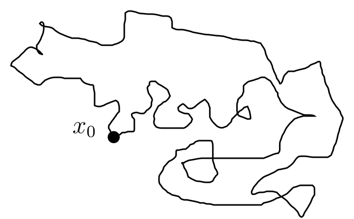
A typical path in the path integral for the partition function. It is a closed path that begins and ends at x_0. — Figure 6:A typical path in the path integral for the partition function. It is a closed path that begins and ends at $x_0$ .

Suppose now that the temperature $T$ is high, so $\beta$ is small. Then the path $x(u)$ cannot deviate very far from the initial condition $x(0)=x_0$ in the short “time” $u=\beta\hbar$ , because if it does it must have a large velocity and that will cause the integral of the kinetic energy to be large which will suppress the integrand exponentially. Therefore as a first approximation let us set $V(x)=V(x_0)$ in the integral in the exponent. Then the integral of the potential energy term becomes

\int_0^{\beta\hbar} V(x_0)\,du = \beta\hbar V(x_0),

(127)

which gives a factor $e^{-\beta V(x_0)}$ in the path integral. But this is independent of the path and can be taken out of the path integral. The path integral that remains is that of a free particle with $t=-i\hbar\beta$ ,

C\int_{x_0\to x_0} d[x(u)] \exp\Bigl[-{1\over\hbar} \int_0^{\beta\hbar} {m\over 2} \Bigl(\dod{x}{u}\Bigr)^2 \, du\Bigr] = \matrixelement{x_0}{U_0(-i\beta\hbar)}{x_0} = \sqrt{\ds{\ds m\over\ds 2\pi\beta\hbar^2}},

(128)

where $U_0$ refers to the free particle, and where we have used (12). Finally, the partition function becomes

Z(\beta) = \sqrt{\ds{\ds m\over\ds 2\pi\beta\hbar^2}} \, \int dx_0 \, e^{-\beta V(x_0)}.

(129)

This result is most easily obtained by classical statistical mechanics. It was known to Boltzmann. By taking into account larger deviations of the path from its initial point we can find quantum corrections to the partition function (effectively expanding in powers of $\beta$ ).

Problems¶

Problem 1.

The propagator can not only be used for advancing wave functions in time, but also sometimes in space. Consider a beam of particles of energy $E$ in three dimensions launched at a screen in the plane $z=0$ . The particles are launched in the $z$ -direction. The screen has holes in it that allow some particles to go through. We assume that the wave function at $z=0$ is $\psi(x,y,0) = 1$ when $(x,y)$ lies inside a hole, and $\psi(x,y,0)=0$ when $(x,y)$ is not in a hole. This is what would happen if we took the plane wave $e^{ikz}$ and just cut it off at the edges of the holes. In other words, $\psi(x,y,0)$ is the ``characteristic function’’ of the holes. Suppose also that the region $z>0$ is vacuum. With an extra physical assumption, this information is enough to determine the value of the wave function in the region $z>0$ .

Define a wave number by

k_0 = {\sqrt{2mE} \over \hbar}.

(130)

Then the Schr"odinger equation } $H\psi=E\psi$ in the region $z>0$ can be written

\del^2 \psi + k_0^2 \psi=0,

(131)

where $\psi=\psi(x,y,z)$ . We would like to solve this wave equation in the region $z>0$ , subject to the given boundary conditions at $z=0$ . (131) is called the Helmholz equation.

The same equation and boundary conditions also describe some different physics. If plane light waves of a given frequency $\omega$ are launched in the $z$ -direction against the screen, and if $\psi$ stands for any component of the electric field, then $\psi$ satisfies (131) with $k_0=\omega/c$ . The problem is one of diffraction theory (either in optics or quantum mechanics).

Write the wave equation (131) in the form,

-{\partial^2 \psi \over \partial z^2} = (k_0^2 + \del_\perp^2)\psi,

(132)

where

\del_\perp^2 = {\partial^2 \over \partial x^2} +{\partial^2 \over \partial y^2}.

(133)

(a) Consider now the equation

i\frac{\partial \psi}{\partial z} = -\sqrt{k_0^2 + \del_\perp^2} \, \psi,

(134)

where the square root of the operator indicated is computed as described in A Function of an Observable. Obviously we have just taken the square roots of the operators appearing on the two sides of (132), with a certain choice of sign. Show that any solution $\psi(x,y,z)$ of (134) is also a solution of (132).

The converse is not true, there are solutions of (132) that are not solutions of (134), but the solutions of (134) all have the property that the waves are travelling in the positive $z$ -direction, something we require on the basis of the physics.

Now suppose that in the region $z>0$ the angle of propagation of the waves relative to the $z$ -axis is small. This will be the case if the size of the holes in the screen is much larger than a wavelength. Then $\del_\perp^2$ acting on $\psi$ is much less than $k_0^2$ multiplying $\psi$ , so we can expand the square root in (134) to get

i\frac{\partial \psi}{\partial z} = -\Bigl(k_0 + {1\over 2k_0}\del_\perp^2\Bigr) \psi.

(135)

This is called the paraxial approximation. Now define a new wave function $\phi$ by

\psi(x,y,z) = e^{ik_0z} \phi(x,y,z),

(136)

and derive a wave equation for $\phi$ .

(b) Now write an integral giving $\phi(x,y,z)$ for $z>0$ in terms of $\phi(x,y,0)$ . Suppose for simplicity there is one hole, and it lies inside the radius $\rho=a$ , where

\rho = \sqrt{x^2+y^2}.

(137)

Show that if $z\gg a^2/\lambda$ , then $\phi(x,y,z)$ is proportional to the 2-dimensional Fourier transform of the hole (that is, of its characteristic function). This is the Fraunhofer region in diffraction theory. Smaller values of $z$ lie in the Fresnel region, which is more difficult mathematically because the integral is harder to do.

(c) Suppose the hole is a circle of radius $a$ centered on the origin. Evaluate the integral explicitly and obtain an expression for $\psi(x,y,z)$ for $z$ in the Fraunhofer (large $z$ ) region. You may find the following identities useful:

J_0(x) = {1\over 2\pi} \int_0^{2\pi} d\theta \, e^{ix\sin\theta},

(138)

where $J_0$ is the Bessel function. See Eq.~(9.1.18) of Abramowitz and Stegun. Also note the identity,

\dod{}{x}(xJ_1(x)) = xJ_0(x).

(139)

See Eq.~(9.1.27) of Abramowitz and Stegun.

This problem can be used to calculate the forward scattering amplitude in hard sphere scattering, a topic we will take up later.

Problem 2.

In classical mechanics, any two Lagrangians that differ by a total time derivative produce the same equations of motion. For example, in one dimension, $L$ and $L'$ , defined by

L' = L + \dod{f(x,t)}{t} = L + \frac{\partial f}{\partial t}+\xdot\frac{\partial f}{\partial x},

(140)

give the same equations of motion. This is easily verified by using both $L$ and $L'$ in the Euler-Lagrange equations,

\dod{}{t}\left(\frac{\partial L}{\partial \xdot}\right) = \frac{\partial L}{\partial x}.

(141)

(a) Let $L_0$ be the classical Lagrangian for a free particle,

L_0(x,\xdot)= {m\over 2}\xdot^2,

(142)

and $L_g$ be the classical Lagrangian for a particle in a uniform gravitational field (with the $x$ -axis pointing up),

L_g(x,\xdot) = {m\over 2}\xdot^2 -mgx.

(143)

According to the principle of equivalence, motion in an accelerated frame is physically indistinguishable from motion in a uniform gravitational field. Consider a region of space free of gravitational fields, where the particle motion in an inertial frame with coordinate $x$ is described by Lagrangian $L_0(x,\xdot)$ . Let $y$ be the coordinate in a frame that is accelerated at constant acceleration $g$ in the $+x$ direction. Assume that the origins of the inertial frame ( $x$ ) and accelerated frame ( $y$ ) coincide at $t=0$ . Transform $L_0(x,\xdot)$ to the $y$ coordinate, and show that the result is $L_g(y,\ydot)$ plus the exact time derivative of a function $f(y,t)$ . Determine the function $f(y,t)$ .

(b) Let $H_0$ and $H_g$ be the quantum Hamiltonians for a free particle and a particle in a uniform gravitational field,

H_0 = {p^2\over 2m}, \qquad H_g = {p^2\over 2m} + mgx,

(144)

and let $U_0(t)$ and $U_g(t)$ be the corresponding time-evolution operators,

U_0(t) = e^{-iH_0t/\hbar}, \qquad U_g(t) = e^{-iH_gt/\hbar}.

(145)

The propagator for the free particle is

\matrixelement{x_1}{U_0(t)}{x_0} =\sqrt{\ds{\ds m\over \ds 2\pi i\hbar t}} \exp\Bigl[{i\over\hbar}{m(x_1-x_0)^2 \over 2t}\Bigr].

(146)

Use the path integral to find the propagator of a particle in a uniform gravitational field, $\matrixelement{x_1}{U_g(t)}{x_0}$ . Hint: you do not need the detailed, discretized version of the path integral (29); instead, just use the compact form (33) and follow the obvious rules of calculus in manipulating it.

Problem 3.

In this problem we use the van Vleck formula (\eqr\cn.84) to find the propagator for the harmonic oscillator.

(a) For the classical harmonic oscillator with Lagrangian,

L = {m \dot x^2 \over 2} - {m\omega^2 x^2\over 2},

(147)

find values of $(x,x_0,t)$ such that there exists a unique path; no path at all; more than one path. Let $\tau$ be a variable intermediate time, $0\le\tau\le t$ , and assume the path $x(\tau)$ satisfy $x(0)=x_0$ , $x(t)=x$ .

(b) Compute Hamilton’s principal function $S(x,x_0,t)$ for the harmonic oscillator, and verify the generating function relations,

p=\frac{\partial S}{\partial x},\qquad p_0=-\frac{\partial S}{\partial x_0},\qquad H=-\frac{\partial S}{\partial t},

(148)

which are equivalent to (51). Do this for some time $t$ such that there exists only one classical path.

(c) We saw in The Path Integral for the Free Particle that the action is minimum along the classical orbits of the free particle. Let $x(\tau)$ be a classical orbit in the harmonic oscillator, satisfying $x(0)=x_0$ , $x(t)=x$ for given values of $(x,x_0,t)$ . Consider a modified path, $x(\tau)+\delta x(\tau)$ , where $\delta x(\tau)$ vanishes at $\tau=0$ and $\tau=t$ . For the operator $B$ in (88) find its eigenvalues $\beta_n$ and eigenfunctions $\xi_n(\tau)$ . Show that if $t<\pi/\omega$ , then all eigenvalues are positive, and the action is a minimum. For other values of time $t$ , show that the number of negative eigenvalues of $B$ is the largest integer less than $\omega t/\pi$ . Thus, for $t>\pi/\omega$ , the classical path is not a minimum of the action functional, but rather a saddle point.

Problem (d).

Put the pieces together, and write out the Van Vleck expression for the propagator of the harmonic oscillator, $K(x,x_0,t)$ .

Problem (e).

Think of the complex time plane, and consider $K(x,x_0,t)$ for times on the real axis satisfying $0< t <\pi/\omega$ . Analytically continue the expression for $K$ in this time interval down onto the negative imaginary time axis, set $t=-i\hbar\beta$ , and get an expression for the matrix elements of the Boltzmann operator, $\matrixelement{x}{e^{-\beta H}}{x_0}$ for a harmonic oscillator in thermal equilibrium. Take the trace to get the partition function $Z(\beta)$ . See if the answer agrees with the partition function of the harmonic oscillator, as found in your typical book on statistical mechanics.

Problem 4..

The classical Lagrangian for a particle of charge $q$ in a given, external, electric and magnetic field $\Evec(\xvec,t)$ and $\Bvec(\xvec,t)$ is

L(\xvec,\dot\xvec) = {m|\dot\xvec|^2\over 2} +{q\over c} \dot\xvec \cdot \Avec(\xvec,t) - q\Phi(\xvec,t),

(149)

where $\Avec$ and $\Phi$ are related to $\Evec$ and $\Bvec$ by (70). For generality we allow the fields to depend on time; thus the time evolution operator $U$ depends on two times, $U=U(t,t_0)$ , as in (3). It turns out that the discretized version of the path integral is

\begin{aligned} &K(\xvec,t;\xvec_0,t_0) = \matrixelement{\xvec}{U(t,t_0)}{\xvec_0} = \lim_{N\to\infty} \left( {m\over 2\pi i\hbar\epsilon} \right)^{3N/2} \int d^3\xvec_1 \ldots d^3\xvec_{N-1} \end{aligned}

(150)

\begin{aligned} &\qquad \times \exp \Bigl\{ {i\epsilon\over\hbar} \sum_{j=0}^{N-1} \Bigl[ {m(\xvec_{j+1} - \xvec_j)^2 \over 2\epsilon^2} +{q\over c} {(\xvec_{j+1} -\xvec_j) \over \epsilon} \cdot \Avec\Bigl( {\xvec_{j+1} + \xvec_j \over 2} \Bigr) -V(\xvec_j) \Bigr] \Bigr\}. \end{aligned}

(151)

The interesting thing about this path integral is that the vector potential $\Avec$ is evaluated at the midpoint of the discretized interval $[\xvec_j,\xvec_{j+1}]$ . Use an analysis like that presented in Equivalence to the Schr"odinger Equation to show that this discretized path integral is equivalent to the Schr"odinger equation for a particle in a magnetic field. Show that this would not be so if the vector potential were evaluated at either end of the interval $[\xvec_j,\xvec_{j+1}]$ (it must be evaluated at the midpoint). Show that it does not matter which end of the interval the scalar potential is evaluated at.

The delicacy of the points at which the vector potential must be evaluated is related to the fact that the action integrals in the exponent of the Feynman path integral are not really ordinary Riemann sums, because the paths themselves are not differentiable. Instead, they obey the $\Delta x \sim (\Delta t)^{1/2}$ rule discussed in the notes. Casual notation such as (33) glosses over such details.

Problem 4.

Let us write the path integral for a charged particle moving in given electric and magnetic fields $\Evec(\xvec,t)$ and $\Bvec(\xvec,t)$ , given in all detail in Eq.~(\eqr\cn.141), in a simplified notation,

K(\xvec,t;\xvec_0,t_0) = C \int d[\xvec(\tau)] \, \exp\Bigl[{i\over\hbar} \int_{t_0}^{t_1} L\bigl(\xvec(\tau), {\dot\xvec}(\tau),\tau\bigr)\, d\tau\Bigr],

(152)

similar to (33), where $L$ is given by (149). Write down a similar expression for $K'$ , which is expressed in terms of vector and scalar potentials $\Avec'$ and $\Phi'$ , where the primed and unprimed potentials are related by the gauge transformation (86), and find the relationship between $K$ and $K'$ . Then given that $K$ is used to advance a wave function $\psi(\xvec,t)$ in time, and $K'$ is used to advance a wave function $\psi'(\xvec,t)$ , find the relationship between $\psi$ and $\psi'$ . Compare to (88).