30. Helium and Helium-like Atoms
Introduction
In these notes we treat helium and helium-like atoms, which are systems consisting of one nucleus and two electrons. If the nuclear charge is , then we are dealing with ordinary helium, while is the ion, is the ion, etc. In recent years there has been some interest in helium-like uranium, the ion , with , for tests of quantum electrodynamics. A case not to be overlooked is , a system consisting of a hydrogen nucleus plus two electrons. This system certainly has unbound states, for example, the states in electron-hydrogen scattering. It is not obvious that it possesses bound states, however, since it is not clear that one proton is capable of binding two electrons. In fact, a bound state of this system does exist, the ion, which can be thought of as an electron bound to an otherwise neutral hydrogen atom. The second electron is rather weakly bound, as we shall see. The ion plays an important role in applications, for example, in energy transport in stellar atmospheres. It is also used in proton accelerators to defeat Liouville’s theorem in the process of filling up accelerating rings. In the following discussion of helium-like atoms we focus mostly on the bound states, but some attention is also given to the unbound states.
The Basic Hamiltonian
In these notes we work in atomic units, . We place the nucleus of charge at the origin of our system of coordinates and we let and be the positions of the two electrons. Then the basic Hamiltonian describing the helium-like system is
where , , and .
This Hamiltonian incorporates all the nonrelativistic, electrostatic effects in helium, but it omits a number of small effects and makes some approximations. The approximation in the use of the Hamiltonian (1) is numerically quite good, but there is some interesting physics in the neglected terms and consideration of them leads to an improved understanding of some of the steps we take in solving the approximate system.
First, the frame attached to the nucleus is not really an inertial frame, since the nucleus is pulled by the electric forces from the electrons and accelerates somewhat in response. The accelerated nucleus then has an effect back on the electrons, so that the overall effect is to couple the dynamics of the electrons. However, since the mass of the nucleus is large in comparison to the mass of the electron, the corrections, which are known as “mass polarization” terms, are small. See Prob.~\cenforce.4, where it is shown that the coupling is proportional to . Similar corrections result from ignoring the small difference between the true electron mass and the reduced mass of the electron and the nucleus. Both these corrections are of order of the electron to nucleus mass ratio, which is approximately 10-4 in helium.
Second, there are a variety of fine structure terms which, as in hydrogen, can be thought of as relativistic corrections. These are all of order or , and are roughly of order 10-3 to 10-4 in helium. (But as in hydrogen, fine structure effects grow with , and are more important in heavier atoms.) In addition to the relativistic kinetic energy correction, the Darwin term and the spin-orbit term, all of which are present in hydrogen, there are also terms representing the interaction of one electron with the magnetic field produced by the orbital motion of the other electron (spin-other-orbit terms), or produced by the magnetic moment of the other electron (spin-spin terms). There are also terms taking into account retardation in the communication between the two electrons.
Third, there are interactions with the quantized electromagnetic field, generalizations of the Lamb shift in hydrogen.
Finally, there may be hyperfine interactions between the electron and the multipole moments of the nucleus (but not in ordinary helium, since the -particle has spin 0).
With the neglect of all these small terms, the basic helium-like Hamiltonian (1) is a purely spatial operator, and does not involve the spin. Thus, it is similar in its level of approximation to the electrostatic model of hydrogen. Due to the requirements of the symmetrization postulate, however, spin plays a significant role in the structure of helium, much more so than in hydrogen at a similar level of approximation.
Wave Functions and Hilbert Spaces
As explained in \jjcouple.3, the Hilbert space of a single electron can be written , where a basis in is the set of position eigenkets and a basis is is the set of eigenkets of the operators and , where and . The quantum number is constant and can be suppressed if it is understood, so sometimes we write simply for the spin eigenkets. A basis in the total Hilbert space is the product basis where . A wave function in the orbital Hilbert space is , while one in the total Hilbert space is .
In a system with two electrons the total Hilbert space is the product of two copies of the orbital and spin Hilbert spaces for the two electrons,
where the numbers in parentheses are the labels of the two electrons. This is the “nominal” Hilbert space discussed in 29. Identical Particles, that is, it consists of the wave functions that we would have if there were no symmetrization postulate. A basis in is the product of the bases in the constituent spaces,
If we rearrange the factors in (2) we can write the total two-electron Hilbert space as
where
The factorization (4) is useful for the study of helium and many other systems with two identical particles. A basis in is the set , while there are two obvious bases in , the uncoupled and coupled,
as explained in \identpart.8. Here is the singlet state and indicates the set of triplet states.
(4) means that an arbitrary wave function in is a linear combination of products of wave functions in and those in . In the special case that a wave function in consists of a single product of this type, we can speak of the “spatial part” and “spin part” of the wave function. Such language is very common in discussions of helium and other two- or multi-particle systems, but it is important to realize that it only applies to wave functions of a special type. The reason such wave functions are relevant in the case of helium has to do with the exchange operators that commute with the Hamiltonian (1).
Exchange Operators
The Hamiltonian (1) commutes with three exchange operators that we now define, in terms of their action on the basis kets in . These are
We will denote the eigenvalues of these three operators by , , and , respectively.
The Hamiltonian (1) commutes with because it is a purely orbital operator that is symmetrical in the exchange of the two electrons. It commutes with because it is a purely orbital operator that commutes with any spin operator. And in view of (11), the Hamiltonian (1) also commutes with .
But the Hamiltonian (1) is only an approximation to the true Hamiltonian for helium. If we include the fine structure terms, which as in hydrogen couple the spin and orbital degrees of freedom, then the resulting Hamiltonian no longer commutes with or separately.
It still commutes with , however, regardless of how many physical effects we include or how many correction terms we add, because the two electrons are identical. All physical Hamiltonians that describe two electrons commute with ; if this were not true, it would be possible to distinguish the electrons.
The properties of these exchange operators follow immediately from their definitions. The operators are all Hermitian and unitary, their square is 1 (the identity operator), and their eigenvalues are , as in (3) and (4). They also satisfy
and
Thus and possess a simultaneous eigenbasis. Since is a function of and , any simultaneous eigenspaces of and is automatically an eigenspace of , with eigenvalue
Since the set of operators are mutually commuting, they possess a simultaneous eigenbasis. Here is the Hamiltonian (1). Equivalently, we can organize the eigenstates of so that they are also eigenstates of and .
To construct such eigenstates we start with . Let us use a capital to refer to states in and a lower case for states in . Then an eigenstate of is the product
for any , since
where the eigenvalue is defined by (47). The most general eigenstate of is a linear combination of such states (14) with the same value of .
Next, we make an eigenstate of by requiring that the spatial part of be an eigenstate of , regarded as a purely orbital operator. That is, we must solve
or, in wave function language,
a purely orbital eigenvalue-eigenfunction problem. This is the hard part, something we shall devote some attention to in these notes.
Then, to obtain an eigenfuction also of , we note that if is a solution of (17), then so is , with the same energy. Thus we can form the wave functions
which, if they do not vanish, are eigenstates of with eigenvalue (the same ± that appears in (18).
Finally, in view of (13), only those states that are symmetric under spatial exchange and antisymmetric under spin exchange, or vice versa, are antisymmetric under total exchange , as required by the symmetrization postulate. The physical subspace of the nominal Hilbert space is the direct sum of the subspace with and , and the one with and .
The situation regarding spatial and spin exchange symmetries is summarized in Table 1, which also indicates some standard nomenclature. As in Table 1, “para” refers to a wave function that is spatially symmetric, and “ortho” to one that is spatially antisymmetric under exchange. At one time helium was thought to consist of two different species, parahelium and orthohelium, since the spectrum of helium indicates two classes of energy levels with no (or only very weak) transitions between them. Table 1 is almost exactly the same as Table 1, the main difference being that in the case of the hydrogen molecule, it was possible to write down an explicit form for the spatial part of the energy eigenfunctions, (33), since we had a central force Hamiltonian, whereas in helium it is much more difficult to solve the spatial eigenfunction equation (16). (And in the hydrogen molecule we had two identical protons, whereas in helium we have two identical electrons.)
Table 1:Linkage of spatial and spin exchange symmetry in helium and terminology.
name | degen | name | ||||
|---|---|---|---|---|---|---|
+1 | para | -1 | -1 | 0 | 1 | singlet |
-1 | ortho | +1 | -1 | 1 | 3 | triplet |
In summary, we have derived the rule about helium eigenfunctions that most students learn in first courses on quantum mechanics, namely, that these eigenfunctions are products of spatial wave functions times spin wave functions with opposite symmetry under exchange. We saw the same rule previously in connection with the hydrogen molecule.
However, the true nature of this rule should be understood. First, the operators and do not have the same fundamental significance as the overall exchange operator . In particular, there is no symmetrization postulate for or . Next, the factorization of the energy eigenfunctions into symmetric spatial parts and antisymmetric spin parts, or vice versa, arises because commutes with and and because commuting operators possess simultaneous eigenstates. If we had included the small fine structure corrections in the Hamiltonian (1), however, then we would find that no longer commutes with or separately, although of course it would still commute with . Thus, the usual rule about the factorization of the wave functions only applies to the nonrelativistic, electrostatic approximation to the helium atom. This is in contrast to the symmetrization postulate itself, which is rigorously correct.
Good Quantum Numbers
Sometimes an operator that commutes with the Hamiltonian is called a “good quantum number.” The terminology is old and it confuses an operator with its quantum number, but it is in common use.
The helium Hamiltonian (1) is not exactly solvable nor even close to any exactly solvable system (at least for small ), so it is rather difficult to obtain good approximations to its eigenstates and eigenvalues. In cases like this it is especially important to pay attention to the exact symmetries of the Hamiltonian, that is, the operators that commute with it (the “good quantum numbers”). Commuting operators possess simultaneous eigenbases, and, since symmetry operators are usually easier to diagonalize than Hamiltonians, it is usually a good idea to diagonalize them first. This means that we need only search in the eigenspaces of the symmetry operators for the eigenstates of the Hamiltonian, a significantly easier task than searching in the whole Hilbert space. For example, if we must diagonalize a matrix to find the energy eigenstates and eigenvalues, it is best to use a symmetry-adapted basis (one that is already an eigenbasis of the symmetry operators). Even if we do not attempt to find the eigenstates of the Hamiltonian explicitly, we can at least say that those eigenstates are labelled by symmetry labels, namely, the quantum numbers of the symmetry operators. This is a common situation for example in particle physics or nuclear physics, where no one knows how to calculate the masses of the baryons or the energies of nuclear states very accurately, but these states are rigorously characterized by their quantum numbers (spin, parity, etc.)
For the helium Hamiltonian (1) we have already begun this process, by noting that commutes with and , and by finding the simultaneous eigenbases of these two operators. This served the dual purpose of narrowing the spaces in which we need to search for energy eigenstates, and of satisfying the symmetrization postulate (by requiring ).
But there are other symmetries of the Hamiltonian (1). Most notably, since is a scalar operator, it commutes with rotations. In fact, since it is a purely spatial operator, it commutes with both spatial and spin rotations independently, and thus with and . It does not, however, commute with spatial rotations of particle 1 or of particle 2 separately, because the term in the Hamiltonian is only invariant when we rotate the positions of both particles simultaneously. That is, does not commute with or separately. The Hamiltonian does commute with and separately, however, in fact, it commutes with any function of spin. But as we have seen, the total spin is more convenient to work with than the individual spins because it is physical and commutes with , and because the coupled basis is an eigenbasis of .
The Hamiltonian (1) also commutes with parity , a purely spatial operator that acts on the basis kets of the entire Hilbert space by
Parity flips the spatial coordinates of the particles but has no effect on spin (at least in nonrelativistic quantum mechanics). We will not make much use of parity in the case of helium, but it is more important in multielectron atoms.
Table 2:Operators that commute with the approximate helium Hamiltonian (\eqr\cn.1) and their corresponding quantum numbers. The symmetrization postulate forces .
Operator | |||||||
|---|---|---|---|---|---|---|---|
Qu. Num. |
A list of operators that commutes with along with their quantum numbers is shown in Table 2. Moreover these operators commute with each other. Thus, without knowing anything else about the eigenstates of , we can say that they are characterized by the quantum numbers of the operators in the table. However, several of the quantum numbers are superfluous. For example, is forced to be -1 by the symmetrization postulate, so and are opposite one another and not independent. In fact, by (46) knowledge of implies knowledge of and therefore knowledge of . Thus an independent set of quantum numbers is . Within a simultaneous eigenspace of the symmetry operators with the given quantum numbers, we can in principle diagonalize the Hamiltonian, and label the energy eigenstates within that subspace by a sequencing number . Thus, the energy eigenstates can be denoted . As for the energy eigenvalues, they are independent of and because of the rotational invariance of the Hamiltonian, so we can write
The energies are -fold degenerate, because of the freedom in the magnetic quantum numbers.
You might suspect that the energies should also be independent of the total spin , since the Hamiltonian (1) is a purely spatial operator. That would be true if there were no symmetrization postulate, but in that case the quantum number would not be superfluous, and, since is a spatial operator itself, the energies would depend on its eigenvalue. In fact, this is precisely what happens in real helium where the symmetrization postulate is operative, it is just that the quantum number is not explicitly stated since it is determined by the value of . In other words, in real helium, the spin state specified by determines the exchange symmetry of the spin part of the wave function which determines the exchange symmetry of the spatial part of the wave function which does affect the energy. Thus, the energy does depend on , in spite of the fact that is a purely spatial operator.
In fact, the dependence of the energy on is typically large, that is, of the order of a Coulomb (electrostatic) energy, much larger than the (magnetic) energies associated with the explicitly spin-dependent terms that we have neglected in Hamiltonian (1). This is because wave functions that are symmetric or antisymmetric under spatial exchange have very different distributions of probability in three-dimensional space, and therefore correspond to quite different Coulomb energies. We will see this explicitly below when we analyze helium by perturbation theory. A similar phenomenon occurs in ferromagnetism, where the energies involved in flipping spins (the magnetization of the material) are much larger than can be accounted for by the magnetic interaction of arrays of magnetic dipoles. This discrepancy in energy scales was known before quantum mechanics had matured, and was regarded as a mystery. The true explanation was given by Heisenberg: when you flip spins, you change the symmetry of the spin part of the wave function, which by the symmetrization postulate forces changes in the spatial part of the wave function, which changes the Coulomb energy of the charge configuration. Ferromagnets are more complicated because there is a large number of particles, but the basic idea is the same as in helium.
In Table 2 we have listed all the obvious symmetries (except parity) of the basic helium Hamiltonian (1). Are there any more (not so obvious) symmetries? Sometimes a system does have additional symmetries in addition to the obvious ones. Notably this happens in the case of hydrogen, which has an symmetry (only the symmetry under spatial rotations is obvious). This extra symmetry is responsible for the extra degeneracy of hydrogen, in comparison to other central force problems. As we say, hydrogen has “hidden” symmetry. Another example with hidden symmetry is the multidimensional, isotropic harmonic oscillator. Apart from these two examples, however, there are very few systems in the real world with extra or hidden symmetry (it depends partly on your definition of “hidden,” but you should not expect such symmetry in most problems). In particular, helium has no extra symmetry beyond what we have listed.
The standard spectroscopic notation for the level is , where is replaced by one of the code letters, , , , , etc., for , etc. As we did in our discussion of the hydrogen molecule in The Hydrogen Molecule, we use capital letters are used to represent the quantum numbers of the collective system (in this case, the whole atom), and reserve lower case letters for the quantum numbers of a single particle (in this case, an electron). For example, the state is the state with , and . This is really a manifold of degenerate states.
Ionization Potentials
So far we have succeeding in labeling the energy levels of helium-like atoms by their good quantum numbers and determining their degeneracies, in the approximation given by (1), without knowing much about the system apart from its symmetries. We now look at some experimental and other facts about such atoms.
First we present some ionization potentials. The ionization potential of an atom is the energy needed to remove one electron from the atom, assumed to be in its ground state, to infinity. If an atom has several electrons, there are successive ionization potentials, as more and more electrons are removed. The final state consists of a nucleus plus the electrons, all of which are at rest and at an infinite distance from one other.
It is a matter of convention in most areas of physics to decide where on the energy axis lies, since only energy differences are physically meaningful. (This is true as long as gravitational effects are neglected. But in general relativity, the mass corresponding to energy by has a gravitational effect, so the absolute measure of energy is physically significant.) But it is common in electrostatics to define the state of zero potential energy to be the one in which all charges are at an infinite separation from one another. This is what we have done with the potential energy in the Hamiltonian (1). If the kinetic energies also vanish, then we have a state of zero total energy. With this convention for the state , the sum of all the ionization potentials of the atom (with a minus sign) is the ground state energy of the atom. (Notice that we have not separated the protons in the nucleus or transported them to infinity. We are using a convention that is convenient in atomic physics, but perhaps not nuclear physics.)
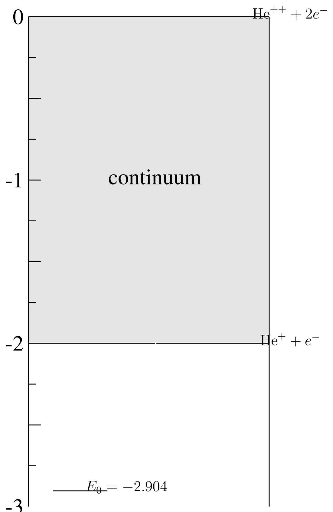
Figure 1:Important energies of helium obtained from ionization potentials. Energies are measured in atomic units.
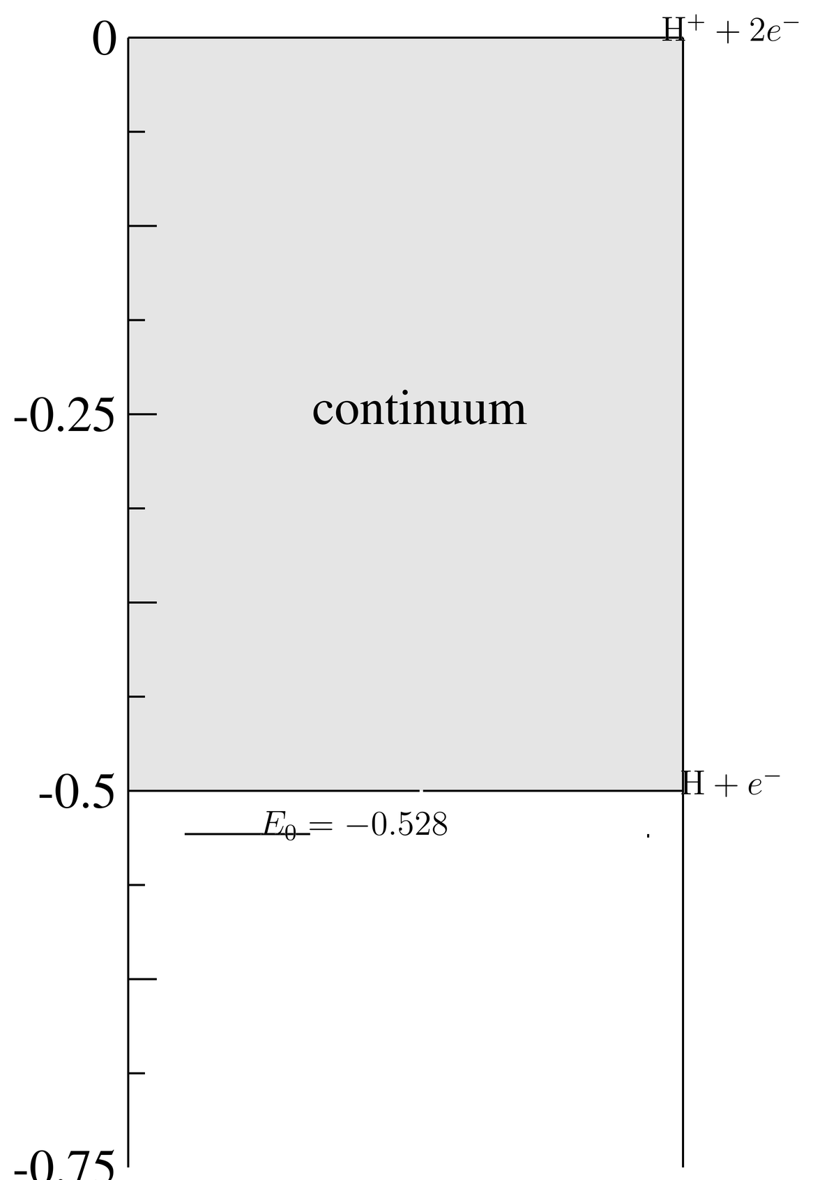
Figure 2:Same as Figure 1, but for . The energy scale is down by a factor of compared to helium.
In the case of helium, the ionization potentials are
The first ionization potential may be compared to that of hydrogen, which is In fact, helium has the highest ionization potential of any neutral atom. See Fig.~\figr\hartfock.1. The second ionization potential is easy to understand, since the ion is a hydrogen-like atom, whose ground state energy is To calculate the first ionization potential, however, is a nontrivial problem. In the case of , the ionization potentials are
In the extra electron is only weakly bound to the neutral H atom.
Figures~Figure 1 and Figure 2 illustrate the information obtained from the ionization potentials. The energy is the state of complete dissociation. The ground state energy of helium is , while the state in which one electron has been removed to infinity has energy Once this electron has been removed, it may be given any positive kinetic energy, so there is a continuous spectrum above In , the ground state energy is and the continuum begins at , the ground state energy of a neutral hydrogen atom.
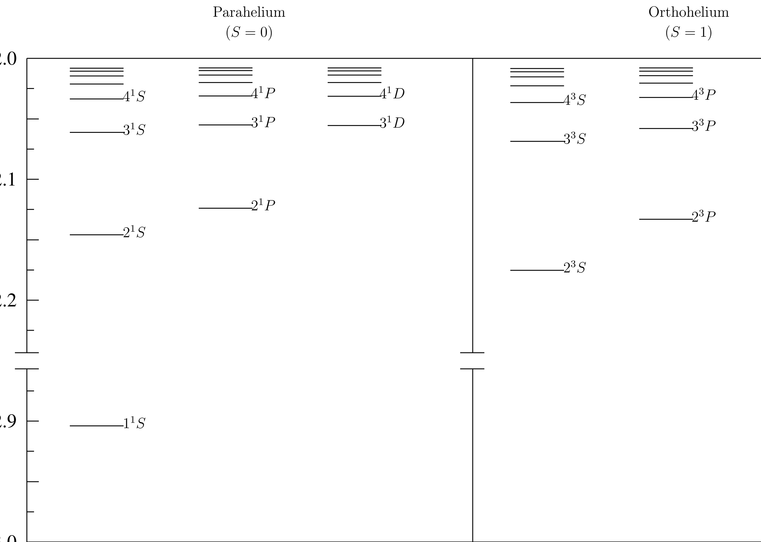
Figure 3:Bound states of helium with quantum numbers. Energies are measured in atomic units. Notice the gap in the energy scale between the ground state and the excited states.
The Bound States
From Figure 1 it is clear that the bound states of helium must lie between and These bound states and their quantum numbers are displayed in Figure 3 with an expanded energy scale. The energy levels in the figure are the eigenvalues of the Hamiltonian (1), which are not exactly the same as the experimental values due to the neglect of small terms in that Hamiltonian. The difference, however, is too small to see on the scale of the diagram (in fact, at higher resolution, many of these levels will be seen to have a fine structure splitting).
The levels in Figure 3 cannot be regarded as purely experimental data, even at a scale where fine structure is ignored and the Hamiltonian (1) is a good approximation, because spectroscopic data only gives differences between energy levels, not their absolute values. It takes some disentangling of the experimental data to produce energy levels. In addition, the levels in Figure 3 have been assigned quantum numbers, which requires some theoretical input. In effect, we have skipped ahead to the answer (the spectrum of helium) in presenting Figure 3. This may be the best way to understand helium on a first pass.
In Figure 3, the para states (spatially symmetric, spin singlet) are on the left, and the ortho states (spatially antisymmetric, spin triplet) are on the right. Each vertical column contains the energy levels for a given value of and , the good quantum numbers of the Hamiltonian (1). Only columns out to (-states) are shown in the figure, but in actual helium ranges from 0 to . The levels in a given column are sequenced in ascending order by , with certain conventions for the starting value of . In each column there is an infinite number of levels that accumulate just below the continuum limit, much as in hydrogen. The energy levels in a given column are the eigenvalues of the Hamiltonian (1), restricted to a simultaneous eigenspace of the operators , , and (it being understood that we are within the antisymmetric eigenspace of the exchange operator ).
Notice the following qualitative features of the energy level diagram for helium. First, the ground state is a singlet state (), which is considerably below the excited states (notice the gap in the energy scale). The excited states look roughly the same on the para and ortho sides, but there is no state (no state on the ortho side that seems to correspond to the state). Second, for a fixed value of and , the energies are an increasing function of (the “staircase effect”) (at least this is true for and most other values of ). This is the same effect we saw in alkali atoms. Third, for fixed and , the ortho states are lower in energy than the para states (thus, if a state existed, we would expect it to be below the actual ground state ). Later we will provide a theoretical explanation for some of these features.
In the case of , the ground state is the only bound state, and it has the quantum numbers (same as the ground state of helium).
Perturbation Analysis. The Unperturbed System
We now turn to the problem of finding the spatial eigenfunctions of the Hamiltonian (1), which is a purely orbital operator. Denoting such an eigenfunction by , we wish to solve
In addition, we wish these eigenfunctions to be even or odd under orbital exchange,
where the is , the eigenvalue of . As explained above, are called para states, and are called ortho states. We know it is possible to construct simultaneous eigenfunctions of and because they commute. Once we have found these eigenfunctions, it will be easy to multiply them by spin states (singlet or triplet) of the opposite exchange symmetry to obtain an overall eigenfunction of the Hamiltonian, including spin, that satisfies the symmetrization postulate. This part is relatively easy; the hard part will be solving (23) as a purely orbital problem.
An obvious strategy for finding the eigenfunctions of the Hamiltonian (1) is to use perturbation theory, in which the inter-electron Coulomb potential is taken as a perturbation. That is, we write , where
We have grouped the terms in to emphasize that is the sum of two hydrogen-like Hamiltonians, one for each electron, moving in the field of a nuclear charge . This decomposition of into and is not very favorable for perturbation theory in the case of small , since the inter-electron potential is comparable to the electron-nucleus potentials. The comparison is especially unfavorable for (the case ). It gets better for larger . We do the perturbation analysis anyway, since it is relatively straightforward and there are not many choices.
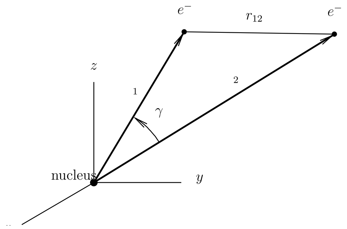
Figure 4:Coordinates for the nucleus and two electrons in space.
It is obvious from Figure 4 what the effect of the perturbation is. When it is switched off, the two electrons no longer repel one another and settle in somewhat closer to the nucleus than they would otherwise. The wave functions for the two electrons can be thought of as two clouds that overlap in the neighborhood of the nucleus. Conversely, when we turn the perturbation on, the electron clouds expand somewhat so the electrons can get away from one another. They also tend to stay on opposite sides of the nucleus, for the same reason.
As usual in perturbation theory, we must understand the unperturbed system first, its eigenfunctions, degeneracies, and symmetries. Since is a sum of two hydrogen-like Hamiltonians, the (two-particle) eigenfunctions of are products of single particle eigenfunctions of the hydrogen-like Hamiltonians in the field of nuclear charge . We call these single-particle eigenfunctions orbitals. They are central force eigenfunctions, and since we are only concerned with the spatial part here, they are characterized by the usual central force quantum numbers . Notice that we are using lower case letters for the quantum numbers of a single electron. The single particle hydrogen-like energy is . We denote these orbitals in ket language by . Then the two-particle eigenfunctions of are products of these, which we denote by
where the numbers in parentheses indicate which of the two electrons (1 or 2) is referred to, and where the right hand side is a shorthand notation for these states. These states depend on six quantum numbers. They are eigenfunctions of ,
where the on the energy indicates that it is the energy in zeroth order of perturbation theory. This zeroth order energy is a sum of the two hydrogen-like energies,
and it depends only on the two principal quantum numbers and .
The states (27) are eigenstates of , but not in general of . However it is easy to construct eigenfunctions of simply by symmetrizing or antisymmetrizing under exchange. There are two cases. In Case I, the two sets of single particle quantum numbers are equal (all of them), , and we write simply
for these states. In this case the states are already even under orbital exchange, so they are para states (). There are no ortho states in Case I.
In Case II, one or more of the two sets of quantum numbers are different, . In this case we can easily write down normalized eigenstates of ,
where the eigenvalue is . In this case we have both para and ortho states. The energy does not change when we carry out this symmetrization or antisymmetrization because both terms have the same energy. It is still given by (29), and it does not depend on the choice of the ± sign. We now have a set of unperturbed energy eigenstates that are also eigenstates of .
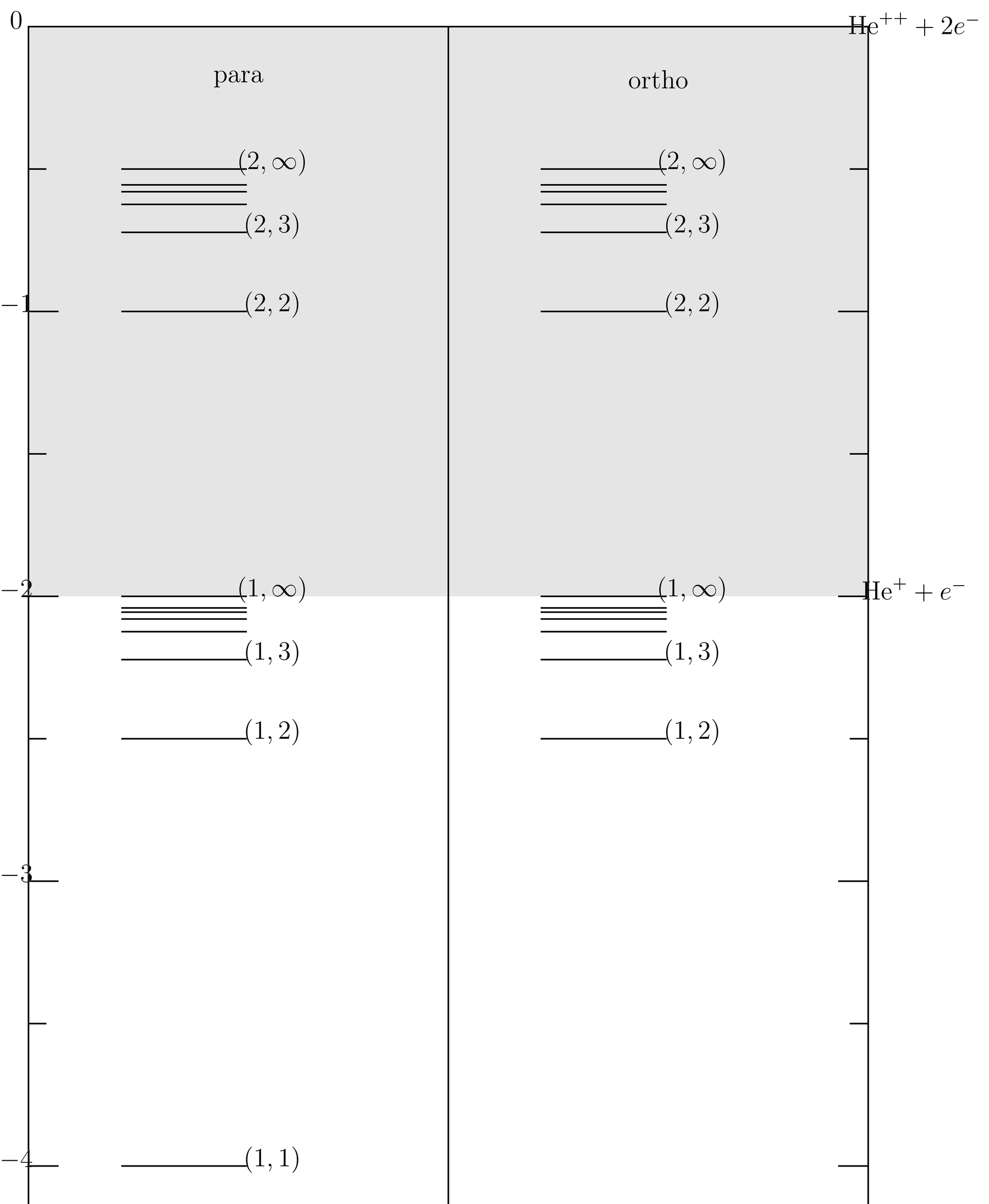
Figure 5:Unperturbed energy levels of helium, that is, levels of the Hamiltonian (25). The energy axis is vertical with energies measured in atomic units, and levels are labeled by principal quantum numbers . The shaded area is the continuum.
Figure 5 shows the energy levels of , with the para states on the left and ortho states on the right. The levels are labeled by their principal quantum numbers .
Let us focus first on the levels below the shaded area in Figure 5, that is, the levels lying below the continuum threshold at (all energies are in atomic units). These levels are called singly excited states because one of the hydrogen-like orbitals is in the ground state (), while the other () takes on any value. The absolute ground state of is the state with , at an energy of -4. The ground state is on the para side; there is no analogous state on the ortho side because this is Case~I, described in the paragraph surrounding (30).
It is instructive to compare these levels with the exact bound states of helium, shown in Figure 3. One difference is that the levels in Figure 3 are separated by the quantum number, while those in Figure 5 are not. There is no point in separating the levels of Figure 5 by the orbital angular momentum quantum numbers because the hydrogen-like energies do not depend on them. Apart from that, however, the two energy level diagrams are qualitatively similar. In particular, in both cases we have an infinite number of levels that accumulate at the continuum threshold .
Our analysis of the unperturbed system shows already why there is no state in real helium: it is because it would have to be a perturbed version of an antisymmetrized ground state wave function, and the ground state wave function is spatially symmetric. On the other hand, the unperturbed spectrum shows no evidence of the staircase effect (hydrogen energies do not depend on ), and there is exact degeneracy between the ortho and para sides (when a level exists on both sides). That is, the unperturbed energies do not depend on the ± sign in (31), which represents the spatial symmetry of the wave function. In addition, the unperturbed ground state is rather badly off in energy, -4 instead of the exact value of -2.904. In fact, all the unperturbed energies are too low; this is because the perturbation in (26) is a positive operator, and can only raise energies. These differences between the unperturbed and exact spectra are clarified by perturbation theory.
The Doubly Excited States
Figure 5 shows something else, the so-called doubly excited states in which both orbitals have principal quantum numbers . The doubly excited series with and is shown in the figure (twice, once on the para side and once on the ortho side). There are other series (not shown), with .
Insofar as the unperturbed Hamiltonian is concerned, these are discrete states imbedded in the continuum. That is, a state such as the state is a bound state of with a normalizable wave function, but it exists at an energy that lies in the continuous spectrum of another set of states, those with and the second electron with a positive energy. The wave functions of the continuum are products of the ground state wave function for the first electron times an unbound hydrogen-like solution for the second electron (subsequently symmetrized or antisymmetrized to obtain a definite exchange symmetry). These wave functions are not normalizable, as we expect in the continuous spectrum.
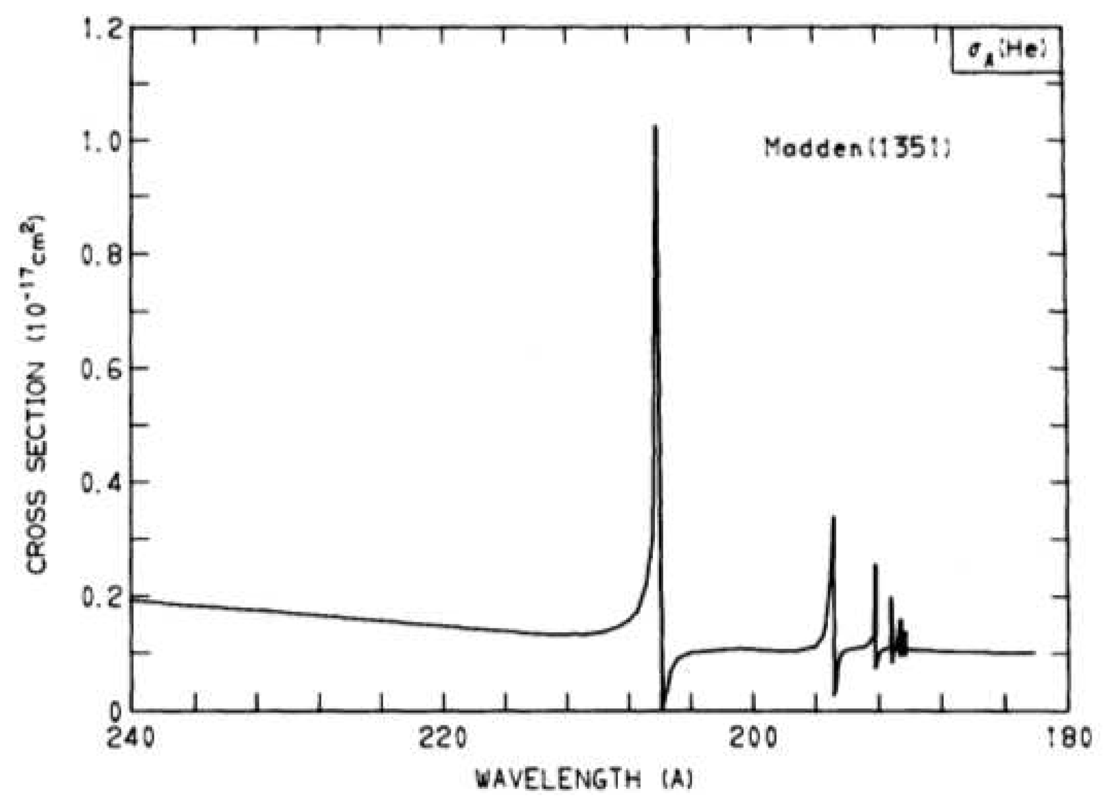
Figure 6:Experimental cross for the reaction , as a function of photon energy. The peaks are resonances corresponding to the doubly excited states of helium. See R. P. Madden and K. Codling, Astrophys. J. 141, 364(1965); and Robert D. Hudson and Lee J. Kieffer, Atomic Data 2, 205(1971).
What happens to these discrete, doubly excited states when the perturbation is turned on? It turns out that they do not remain discrete states, instead they become coupled to the continuum states of nearby energy, so the actual spectrum of helium above the continuum threshold is strictly continuous. There are no exact bound states of helium above this threshold.
Nevertheless, the exact system does in effect know about the doubly excited states of the unperturbed system. Consider, for example, what happens when we direct a beam of photons of some energy at helium atoms in the ground state. When the photon energy exceeds the ionization potential of helium, 0.904~a.u., it may be absorbed by the atom and an electron ejected. The electron emerges with an energy that is the difference between the photon energy and the ionization potential. The experimental cross for this reaction is shown in Figure 6. One can see sharp peaks or enhancements in the cross , which correspond to the doubly excited states of helium. One can view this reaction as a two-step process, , in which refers to a doubly excited state.
This effect can be understood classically. The solar system has eight major planets that move in approximately circular orbits that are stable on human time scales. Nevertheless, it is energetically possible for Jupiter to move somewhat closer to the sun, moving into a lower energy state, and eject all the other seven planets from the solar system. Will this ever happen? Modern chaos theory indicates that it probably will, if we wait long enough, assuming that the motion of the planets is governed by Newton’s laws and no other effects (such as the death of the sun or an encounter with another star) intervene. Nevertheless, the solar system must be mostly stable for very long times, since the earth has apparently been in approximately the same orbit for about years.
Whether or not the ejection of the major planets is possible, it certainly happens that Jupiter and other planets have encounters with other (usually smaller) objects and cause them to be ejected. This effect is deliberately exploited by spacecraft that are to leave the solar system (such as the Mariner spacecraft).
In the case of the doubly excited states of helium, we can imagine the two electrons having a close encounter, which causes one to drop into the ground state and the other to be ejected. Unlike the case of the solar system, where Jupiter can move into any state of (continuous) lower energy, the first electron must drop into one of the discrete energy levels allowed to it. This is why the actual ground state of helium is stable: the two electrons are interacting strongly all the time, but there are no lower states for one of them to drop into. Apart from the effects of quantization, the classical picture gives an idea of the mechanism in helium. In particular, depending on the two sets of quantum numbers of the doubly excited state, it may take a long time for one electron to have a close encounter with the other. This is like the long-time stability of the solar system. In this case we have a state of the system that is nearly a stationary state, that is, an energy eigenstate. It is not exactly a stationary state, however, instead it is a resonance, a state with a finite life time. Resonances were examined in homework problem Paragraph in a simple one-dimensional example.
Helium can be raised into a doubly excited state by many methods, not only absorption of photons but also collisions with electrons or other means. In all cases the doubly excited state exists for a period of time and then decays into the helium ion and a free electron. This is called the Auger process.
Perturbation Analysis of the Ground State
The ground state wave function of is of the form (30), with , that is, it is the state . It is nondegenerate, so to compute the energy shift due to in first order perturbation theory we must compute\
where we have written out the matrix element explicitly as an integral over the six-dimensional configuration space and where the wave functions are hydrogen-like orbitals in the field of nuclear charge .
The integral (32) has an interpretation in electrostatics. The squares of the wave functions seen in that integral are probability densities for the two electrons in physical space, which may be multiplied by the charges ( in atomic units) to obtain charge densities. Then the integral is the mutual energy of interaction of the two charge clouds. That is, if we imagine the two charge clouds translated rigidly, starting at an infinite separation, then the integral is the energy required to bring them into their final position where they overlap completely. Because the charge clouds repel one another, this energy is positive. It is precisely the energy shift in first order perturbation theory.
The hydrogen-like orbital for the ground state is
To do the integral (32) we expand the Coulomb denominator,
where
and
See \orbamsph.11. The angle is illustrated in Figure 4. In addition we expand the Legendre polynomial in (34) in terms of spherical harmonics, using the addition theorem (72). For our present purposes we write this theorem as
Transforming the integral to spherical coordinates in both and and collecting all the pieces, we have
We do the integral first, using the orthonormality of the 's and the fact that is a constant,
The Kronecker deltas cause both sums to be replaced by the single term . Then the integration is easy,
This leaves us with
where is the second integral,
These integrals are elementary and after some algebra we find
or
where the means the energy correct to first order of perturbation theory. Evidently perturbation theory is developing a series in inverse powers of .
Table 3:Comparison of ground state energies at zeroth and first order of perturbation theory with the exact ground state energies, for and .
Atom | ||||
|---|---|---|---|---|
1 | -1 | -0.375 | -0.528 | |
2 | -4 | -2.75 | -2.904 |
Table 3 shows a numerical comparison of the ground state energies of helium and , as estimated from the unperturbed system and from first order perturbation theory. It will be seen that the first order correction does close the gap between the calculated energy and the true energy, but it overshoots the mark and ends up being too high.
If we did not know the exact ground state energy, what would we make of this estimate from first order perturbation theory? For example, do we have any idea how far away it might be from the true ground state energy, or whether it is even too high or too low?
We know that the variational principle always gives us an upper bound to the ground state energy. It turns out that the estimate from first order perturbation theory can be interpreted as a variational estimate, and that it is, therefore, an upper bound. The trial wave function that makes this identification is the unperturbed eigenfunction, which in this case is nondegenerate. See Prob. Paragraph. But perturbation theory alone does not give a lower bound, so we are somewhat in the dark as to how far away our estimate is from the true ground state. In practice we can get information about this by applying variational estimates with more and more sophisticated trial wave functions, and observing the numerical convergence. This is not rigorous, but often it works well enough.
In this example we do have a lower bound, namely, the ground state of , which is -4. This is not very close to the true ground state, nor can we improve the estimate as we can with the variational method, by choosing better trial wave functions. There are methods of getting lower bounds that can be improved, which we do not consider here.
Even without knowing how far away we are from the true ground state, however, an upper bound can be useful for some purposes. Consider, for example, the ion. It is not obvious on physical grounds that this exists as a bound state. If it were not known experimentally that it does exist, how could we prove it theoretically? One way is to find a trial wave function that gives an upper bound to the ground state energy that lies below the continuum threshold, which is Unfortunately, our estimate from first order perturbation theory, , lies above this threshold, so we do not have a theoretical proof of the existence of . But we should keep this example in mind later when we apply the variational method to helium-like atoms.
Perturbation Analysis of the Excited States
We now apply perturbation theory to the excited states of helium, concentrating on the bound states. We need consider only the singly excited states, since, as noted, the doubly excited states are already above the continuum threshold, and the perturbation can only raise the energies. We will set for the singly excited states, so the unperturbed energy is
We will be interested in the case . We write the unperturbed energy eigenstates as
where we use the notation (27) for the products of hydrogen-like orbitals. This is case~II, shown in (31). The ± sign on either side is the eigenvalue of , the orbital exchange operator. As for the notation , we are using capital letters for the quantum numbers of all the electrons in the atom, and lower case letters for the quantum numbers of a single electron. For example, is the quantum number of the operator . But for singly excited states the entire angular momentum comes from the second electron, since the first electron is in the ground state for which . Thus in (46) it is understood that , and . For example, the state with , and is the unperturbed version of the state in helium. Whether we write or depends on which aspect of the problem we wish to emphasize. In any case, notice that the notation contains quantum numbers of the orbital observables in Table 2 that commute with the entire Hamiltonian . That is, we are using a symmetry adapted basis for studying the perturbation.
The unperturbed eigenstates (46) are degenerate, since the unperturbed energy depends only on the quantum number , and we should think about degenerate perturbation theory. But in the basis we need not diagonalize any matrices, since commutes with all the operators of the complete set of commuting observables that specify the unperturbed basis vectors inside a degenerate eigenspace of the unperturbed Hamiltonian, that is, the operators , and . Therefore the energy shifts are given by the diagonal matrix elements,
The energy shifts do not depend on because of the Wigner-Eckart theorem and the fact that is a scalar operator, but they do depend on all the other quantum numbers , as we shall see. Substituting (46) into (47) we have
But the pairs of matrix elements inside the round parentheses are equal, as we see by writing them out as spatial integrals and swapping and , so we have
where
The integrals and are called the direct and exchange integrals, respectively. As for the direct integrals, if we write them out explicitly as a integrals over the configuration space of the two electrons, using the hydrogen-like orbitals , we have
This has the interpretation as the mutual electrostatic energy of the two electron clouds associated with orbitals and , exactly as in the integral (32), which applies to the ground state of helium. In fact, that integral is a direct integral itself, with . The direct integrals are obviously real and positive.
As for the exchange integrals, they are
These are also real, as is easily shown by swapping the variables of integration and . It can also be shown that the exchange integrals are positive. We will omit the proof of this fact since it is not particularly illuminating, but we note that it is plausible that should be positive, since the denominator makes the integrand large in regions of the six-dimensional configuration space where . But in such regions, the numerator is approximately
where . That is, the numerator is positive in such regions. (The rigorous proof that is given in an appendix to Slater’s books on atomic physics.)
The fact that is positive has a simple physical interpretation, however. Since the energy shifts (49) are , it means that the ortho states (with the sign) are lower in energy than the para states (with the sign). This is one of the qualitative features of the exact spectrum of helium noted in The Bound States. One can understand why this is so as follows. Let be the wave function of the two electrons. For ortho states, . But when , this means . For ortho states, the two-electron wave function vanishes when the two electrons are on top of each other, that is, the wave function has a node at . For para states, on the other hand, the wave function has an anti-node, that is, it is a maximum at . (In using the words “node” and “anti-node” we are applying one-dimensional terminology to the six-dimensional problem at hand, but the terminology does convey the right idea.) But since the electrons repel one another and do not like to be on top of one another, the electrostatic energy of interaction is larger in para states than in ortho states.
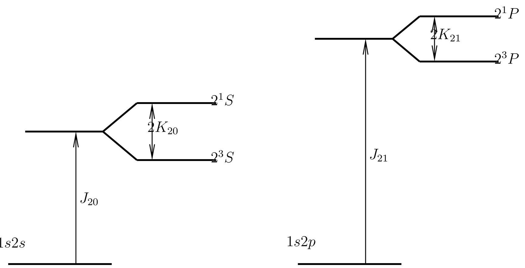
Figure 7:Effect of the perturbation on the levels of helium. Diagram is schematic and not to scale, but it does show the correct ordering of the levels in real helium, that is (from lowest to highest), , , , .
A schematic illustration of the effects of the perturbation on the levels of helium is given in Figure 7. The unperturbed levels are labeled with the quantum numbers of the hydrogen-like orbitals that enter into the unperturbed wave functions, that is, and . Such a list of central force quantum numbers for individual electrons is called an electron configuration of the atomic state. In the same notation, the ground state is given the configuration (both electrons are in the orbital). Notice, however, that the electron configuration applies rigorously only to the unperturbed wave function. For example, although we say that the electron configuration in the ground state of helium is , or that that of the levels is or , nevertheless the exact wave functions are not products of single electron orbitals (in the case of the ground state) or symmetrized or antisymmetrized products (in the case of the excited states). This is because the perturbation changes the wave functions.
A qualitative feature shown in Figure 7 is the fact that the direct integrals are an increasing function of . This is responsible for the “staircase effect,” that is, the fact that the levels are higher than the levels. A similar effect can be seen in the alkalis (see Fig.~\figr\hydrogen.3 for the case of sodium), and the explanation is the same: as the angular momentum of one electron is increased, it moves further away from the nucleus, and the nuclear charge is more effectively screened by the other electron(s) (one, in the case of helium; the core electrons, in the case of the alkalis).
We see that all the qualitative features of the excited states of real helium, discussed in The Bound States, are explained by perturbation theory. These are the absence of any state; the fact that the ortho states are lower in energy than the singlet states; and the fact that the energy is an increasing function of (the staircase effect). From a quantitative standpoint, however, perturbation theory, as we have outlined it, is less satisfactory, which is why we do not attempt to evaluate the direct and exchange integrals explicitly. The variational method does better from a quantitative standpoint.
Variational Treatment of Ground State
The unperturbed ground state was represented in ket language in Perturbation Analysis of the Ground State as . In wave function language it is the product of two hydrogen-like ground state orbitals (see (33),
where the subscript refers to the electron configuration of the ground state. The unperturbed energy (-4) is rather badly off. The reason was explained in Perturbation Analysis. The Unperturbed System: the two electrons repel one another, and the true charge cloud stays somewhat further away from the nucleus than indicated by (55).
Equivalently, we can say that each electron partially screens the nucleus from the other, so that each electron sees an effective nuclear charge that is somewhat less than the true nuclear charge . Since only one electron is doing the screening and the screening is only partial, we would expect any reasonable measure of to lie between and . This suggests that we use as a trial wave function the product of two hydrogen-like ground-state orbitals in a Coulomb field with effective charge , that is,
where we treat as a variational parameter. In accordance with the variational method we will minimize the expectation value of the energy with respect to , and thereby determine . This is an example of how we can use physical reasoning to choose a trial wave function. We will write the wave function (56) in ket language as .
The trial wave function (56) is already normalized, so we do not need any Lagrange multipliers (see Lagrange Multipliers for Normalization). We merely need to calculate the expectation value of . To do this we write in the form,
where we have added and subtracted terms to cause the appearance of two single-particle, hydrogen-like Hamiltonians with nuclear charge .
The expectation value of the first major term in (57) with respect to the trial wave function is
where we have factored the two-particle wave function into a product of two single-particle orbitals, and where the numbers in parentheses indicate which particle is referred to. But the operator in the middle depends only on the coordinates of particle 1, so the bra and the ket referring to particle 2 just combine to give their normalization, which is 1. Thus the two-particle matrix element (59) reduces to a single-particle matrix element,
where we drop the superscripts and 1 subscripts, since the coordinates of the remaining particle are just dummy variables of integration. This is the expectation value of a hydrogen-like Hamiltonian with effective charge with respect to its own ground state, which is just the ground state energy with the same effective charge, as shown. The expectation value of the second major term in (57) proceeds similarly, and gives the same answer, doubling the contribution (60).
As for the third major term in (57), we will need the expectation value of with respect to the trial wave function. This is
where we proceed as in the previous paragraph to reduce the two-particle matrix element to a one-particle matrix element, and where we use (45) for the final expectation value (with replaced by and ). The expectation value of proceeds similarly, and doubles the answer. Overall, the expectation value of the third major term in (57) is
As for the final term in (57), the inter-electron potential , this depends on the coordinates of both particles and so its expectation value cannot be reduced to a single-particle matrix element as in the case of the other terms. However, the expectation value in question is the same one we calculated earlier in our perturbation analysis of the ground state (in Perturbation Analysis of the Ground State) except for the replacement of by . Therefore the answer follows immediately from (43),
Adding up the pieces, we have
We wish to minimize with respect to . We have
which has the root
We see that by the variational criterion of the best trial wave function, each electron screens of a nuclear charge from the other electron. The variational estimate for the ground state energy is where is given by (67). This is
The first two terms agree with the results of first order perturbation theory, (44), but with correction which is negative. Since the variational result is an upper limit to the ground state energy, we see that
where the superscript refers to the results of first order perturbation theory, as in (44).
Table 4:Comparision of ground state energies of and , calculated by both perturbation theory and the variational method, with the exact ground state energies.
Atom | ||||||
|---|---|---|---|---|---|---|
1 | -1 | -0.375 | -0.473 | -0.528 | ||
2 | -4 | -2.75 | -2.848 | -2.904 |
Table 4 summarizes the results of both perturbation theory and the variational method for the ground states of and . In the case of helium we see that the variational method has closed about two thirds of the distance between the results of first order perturbation theory and the exact ground state energy. In the case of the variational result is disappointing, in that the estimate of the ground state energy (-0.473) is still above the continuum threshold of -0.5. If we did not know that exists as a bound state, we would not yet have a theoretical proof that it does. To give that, it would be necessary to find a more complicated trial wave function (with more or different parameters), such that the expectation value of the energy would be less than -0.5. From a physical standpoint, it is clear what is wrong with our trial wave function (56): it does not incorporate the tendency of the electrons to stay on opposite sides of the nucleus, that is, it does not incorporate any correlation in the positions of the two electrons. With a trial wave function that does take this effect into account, it is possible to obtain a variational estimate that is less than -0.5, thereby providing a theoretical proof of the existence of as a bound state.
The variational method has been applied to the ground state of helium and helium-like atoms with much more sophisticated and complicated trial wave functions than we have considered here. The original calculations along these lines were carried out by Hylleraas, and with modern computers it is possible to go much further. By such means the ground state energy of the Hamiltonian (1) for and other values of has been obtained to many significant figures. The accuracy obtained is far beyond that needed to show the difference between the ground state energy of the Hamiltonian (1) and the experimental ground state energy of helium, which are not equal because the Hamiltonian (1) omits a number of small effects, as discussed in The Basic Hamiltonian.
Problems
Problem 1.
The bound states of helium are shown in Fig.~\figr\cn.3.
(a) How would this diagram be different if the electron were a spin~0 particle? If it were a spin~ particle? You do not need to be quantitative, but if some levels go up or down, say which ones and which way. If some levels appear or disappear, say which ones. What are the degeneracies of the levels in actual helium? What would they be if the electron were a spin-0 particle?
(b) The electric dipole operator for a multielectron atom is defined by (12), where the charges are the electrons (with . Electric dipole transitions between two states are governed by the matrix element of the electric dipole operator between the states in question. Explain why there are no electric dipole transitions between ortho and para eigenstates of the Hamiltonian (1).
Remark: The eigenstates of the Hamiltonian (1) are not exactly the eigenstates of real helium because of the neglect of small terms, notably, the fine structure terms. When these are included, it turns out that electric dipole transitions are allowed between ortho and para states, but the amplitude is small and the lines are very weak. For this reason, it was thought at one time on spectroscopic grounds that parahelium and orthohelium were two different species of helium. The weak spectral lines connecting the ortho and para states are called “intercombination lines.”
Problem 2.
This problem was borrowed from Eugene Commins. Consider a simple ``one-dimensional’’ hydrogen atom that obeys the equation,
[Units such that , and the Coulomb potential is replaced by ].
(a) Find the ground state energy and wave function , and verify that
(b) Now consider the one-dimensional “helium” atom which obeys
where , are the coordinates of the two “electrons” on the -axis. First treat as a perturbation and find the ground state energy to first order. Compare to 3-dimensional helium.
(c) Now employ the variational method with a trial wave function analogous to that used in class for the ground state of 3-dimensional helium. Find the best value of and compare to 3-dimensional helium.
(d) For one-dimensional “helium,” take a trial wave function of the form
where is the variational parameter (that is, the whole function, as in Hartree theory). Assume is real; there is no loss of generality in this. Find an equation for . It will be a kind of Hartree equation, and it will contain a pseudo-energy eigenvalue, call it . Define so that the equation looks like
where the ellipsis indicates omitted terms.
(e) The desired solution must be normalizable (in fact, we demand that it be normalized), so we must have
Show that this can only be satisfied if . Hint: To solve the equation, make the change of notation, , , and interpret it as a one-dimensional problem in classical mechanics.
(f) Find the normalized solution and the pseudo-eigenvalue .
(g) Find the variational estimate of the ground state energy of one-dimensional “helium”. Hint: Note that
Does your new estimate improve on the results of part (a)? Would you expect it to do so?
Problem 3.
A problem on the excited states of helium.
(a) The exchange integral defined in (53) depends on two hydrogen-like orbitals. It is easily generalized to any two single-particle orbitals (recall that “orbital” means a single-particle wave function). Show that if the two orbitals have no spatial overlap, then the exchange integral vanishes. Then use your knowledge of hydrogen-like orbitals to explain the dependence of the exchange integral on for fixed , and on for fixed .
(b) Go to {\tt http://