51. Hole Theory and Second Quantization of the Dirac Equation
Introduction
In these notes we provide the ultimate resolution of the difficulty of the negative energy solutions, which appear both in the Klein-Gordon equation and in the Dirac equation. The results are dramatic on several accounts. First, they lead to the physical prediction of the existence of antimatter, something that was not suspected when Dirac began his work on relativistic wave equations. This prediction came only a short time before positrons were found experimentally, in one of the most brilliant theoretical successes in the history of physics. Second, the ultimate resolution of the difficulties of the negative energy solutions shows that in relativistic quantum mechanics, it is impossible to speak of a system consisting of a single particle. Instead, particles and antiparticles are present everywhere and in all circumstances, at least virtually, with observable consequences. And finally, the proper framework for understanding relativistic quantum mechanics appears, and it is not some Schr"odinger-like equation for one or some fixed number of particles, rather it is quantum field theory.
We summarize where we are in our exploration of the Dirac equation. Although we have as yet no interpretation for the negative energy solutions, and although we do not see them physically, we have seen that we cannot simply declare them to be nonphysical. Two reasons were given in The Zitterbewegung: First, the negative energy solutions of bound state problems do not span the same subspace of the Hilbert space as negative energy solutions of the free particle, so there is no consistent way to define a nonphysical subspace; and second, the negative energy solutions seem to be necessary to get the Zitterbewegung, which explains the Darwin term in atoms.
Here is another reason, which involves the fact that the positive energy solutions by themselves do not form a complete set. In second order perturbation theory, it is necessary to sum over a set of intermediate states, as shown by (20). This sum comes from a resolution of the identity, inserted into the terms of the Dyson series, so it must be taken over a complete set of states. But in the case of the Dirac equation, should the sum include the negative energy solutions? If they are nonphysical, it seems we should not.
Let us take an example. If we use the nonrelativistic theory to calculate the cross for the scattering of a photon by a free electron, we obtain the Thomson formula, (60). See also Prob. Paragraph. The Thomson formula comes from the seagull diagram only, since the other diagrams are negligible in comparison. The seagull diagram in turn comes from the second order Hamiltonian (see 43. Scattering of Radiation by Matter{} for the notation), taken in first order perturbation theory, so there is no sum over intermediate states.
Now if we do the same calculation using the Dirac equation, there is no second order Hamiltonian, and the first nonvanishing contributions to the scattering amplitude come from the first order Hamiltonian, taken in second order perturbation theory. Thus there is a sum over intermediate states. But if we exclude the negative energy solutions in this sum, it turns out that we throw away precisely the terms that in the nonrelativistic limit give the seagull graph. Thus, the cross calculated in this limit does not agree with the Thomson formula, which we know is correct. We know this because it is verified experimentally, and, in any case, it can be derived from purely classical electromagnetic theory. We see that the negative energy solutions are needed in sums over intermediate states in order to get physically correct results.
Hole Theory
So we cannot declare the negative energy states to be nonphysical. But there are also problems if we assume that they are real. For example, a real electron interacts with the electromagnetic field, and this is an interaction that we cannot turn off. Consequently an electron in a higher energy state can emit a photon and drop into a lower energy state. This cannot happen with a free electron, because it is impossible to satisfy energy and momentum conservation when emitting a photon and dropping from one free particle state to another. But it can happen in bound systems such as the hydrogen atom, in which the nucleus can absorb any extra momentum needed to satisfy overall energy and momentum conservation. For example, the lowest positive energy eigenstate of the Dirac hydrogen atom is the usual ground state, approximately 13.6~eV below the rest-mass-energy of the electron, . But the Dirac hydrogen atom also has a continuous spectrum of negative energy states, lying in the range . Why, then, cannot a hydrogen atom in the usual ground state emit a photon, and drop into one of the negative energy states? This photon would have an energy close to or higher. Moreover, once one negative energy state has been reached, the system could emit another photon, dropping into an even more negative energy state. This process, it would seem, would continue forever, as the energy of the electron went to , and an infinite amount of energy in the form of photons was released. One can calculate the life time of the (usual) ground state of hydrogen according to this mechanism, and it turns out to be very short. Obviously, we do not see hydrogen atoms self-destructing in this manner and emitting an infinite amount of energy in the form of photons.
In 1930, Dirac suggested that the reason we do not see such transitions is that the negative energy states are already filled. Since electrons are fermions no more than one can occupy a given state, so transitions to negative energy states would be forbidden by the Pauli exclusion principle. These negative energy electrons constitute what is called the “Dirac sea.” According to this hypothesis, space is filled with the sea of negative energy electrons, which produce a nominally infinite density of both energy and negative charge. So we have to imagine some mechanism that would prevent the sea from having observable effects. Perhaps the infinite electric field created would cancel out from symmetry, since there would be no preferred direction for it to point in. And never mind the gravitational effects of the infinite mass density.
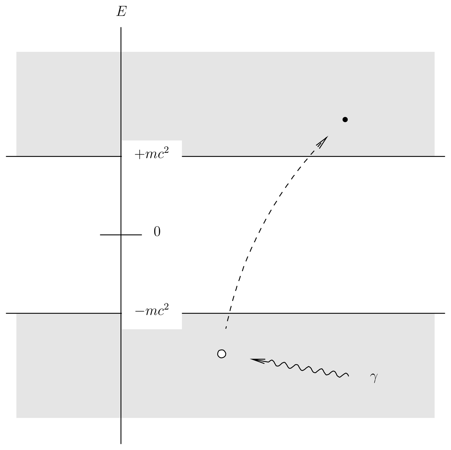
Figure 1:A diagram suggestive of the physics of pair creation, according to hole theory. A photon is absorbed by a negative energy electron, which is promoted into a positive energy state, leaving behind a hole.
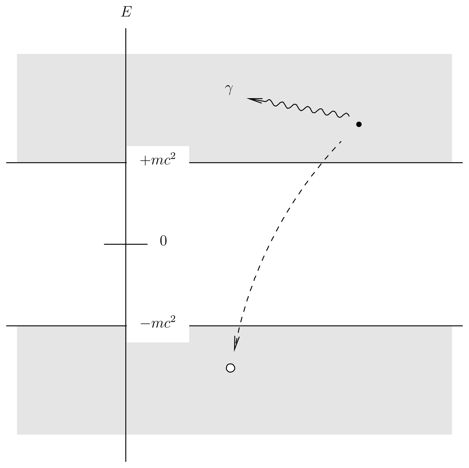
Figure 2:Pair annihilation according to hole theory. A positive energy electron makes a transition to a negative-energy state, filling up the hole and emitting a photon in the process.
Pushing these problems aside, Dirac noted that his hypothesis leads to predictions of new physics. For example, although a positive energy electron could not make a transition to one of the (already filled) negative energy states, the negative energy electrons in the sea also interact with the electromagnetic field, so it is possible for one of them to absorb a photon and get lifted into a positive energy state. The photon would have to have an energy for this to happen. But if it did, we would see the disappearance of the photon, and the appearance of a (regular) positive energy electron that was not there before. We would see something else, too, a “hole” in the negative energy sea, that is, the absence of a negative energy electron. If the electric field of the (normally filled) negative energy sea somehow cancels, then, when we remove a negative energy electron, its electric field no longer contributes to the sum, and now the sum of the field from the negative energy sea would be the negative of the field contributed by the negative energy electron that was removed. That is, we would see the electric field of a particle of positive charge. In fact, the absence of the negative energy electron would behave overall as a particle with the opposite charge, energy, momentum and spin of the negative energy electron, that is, it would have positive energy as well as positive charge. Thus Dirac arrived at the prediction that a photon can disappear and be replaced by an ordinary electron, plus a new particle with the same mass as the electron but opposite charge. This process is illustrated in Figure 1.
Since such a particle had never been observed at the time of Dirac’s 1930 paper, he tried to imagine that it was the proton. Unfortunately, the proton does not have the same mass as the electron, so the whole idea seemed shaky. Pauli was especially skeptical, and criticized Dirac’s theory. In 1932, however, Anderson discovered the positron in cosmic ray tracks, a particle of the same mass as the electron but with the opposite charge, thereby vindicating Dirac. The process described is now called “pair creation” (the creation of a positron-electron pair). A photon cannot create an electron-positron pair in the vacuum, because it is impossible to conserve energy and momentum in the reaction . But if a nucleus is nearby to absorb the extra momentum, then it can happen. In Anderson’s experiment, layers of lead (a high material) were separated by gaps. A high energy photon, created by the interaction of a cosmic ray muon in one of the lead plates, passed down to a lower plate where it produced an electron-positron pair, which emerged into the next lower gap.
Dirac’s “hole theory” also makes other predictions. If a hole has been created in the negative energy sea, then it is no longer impossible for a (regular) positive energy electron to make a transition into that particular negative energy state, emitting a photon in the process. Thus we have the prediction that an ordinary electron and a hole, which is manifested as a positron, may simultaneously disappear, with the appearance of a photon. That is, Dirac’s hypothesis of the negative energy sea leads to the prediction of the reaction, . This reaction cannot occur in vacuum because of energy and momentum conservation (just look at the reaction in the rest frame of the - system and you will see), but an annihilation into two photons, , is possible, and is observed to happen. Thus, Dirac’s hole theory predicts that a hole (otherwise known as a positron) and an electron can annihilate one another, leaving behind only photons. It is a direct conversion of matter into energy, as promised by the Einstein relation . This process is illustrated in Figure 2.
Successes and Shortcomings of Hole Theory
The Dirac equation, combined with the hypothesis of the negative energy sea, constitutes “hole theory.” It not only solves the problem of the negative energy solutions of the Dirac equation, but also forms the basis of a theory that can be used for many sophisticated calculations in quantum electrodynamics. Indeed, it was so used for many years, although it is definitely out of fashion nowadays, and in these notes we shall give it no more than a brief treatment. For us its main importance is as a crucial stepping stone to the modern point of view, which is based on quantum field theory.
In spite of its successes, hole theory also has a number of shortcomings. First, although it describes very well many processes in quantum electrodynamics involving the creation and annihilation of electrons and positrons, it cannot easily describe other processes in which electrons or positrons are created and destroyed, such as beta decay. Consider, for example, the beta decay of a neutron,
where is a proton, an electron, and an antineutrino. This reaction is a manifestation of the weak interactions, not the electromagnetic. If the electron that appears in beta decay is to be interpreted as one that has been promoted out of the negative energy sea, then we would expect to see a positron left behind. Instead, the positive charge is carried by the proton.
In addition, there are a number of theoretical, interpretational and esthetic difficulties with hole theory. For example, the hypothesis of the negative energy sea makes crucial use of the fact that electrons are fermions, so that the exclusion principle can prevent transitions from positive energy states to negative energy states, at least under normal circumstances in which the negative energy sea is filled. Although this resolves the difficulty of the negative energy solutions for the Dirac equation, it does not help with the negative energy solutions of the Klein-Gordon equation, which describes bosons. (The Klein-Gordon wave equation must describe bosons because the wave function is a scalar, which must represent a particle of spin~0.)
There is also the obvious problem of how to understand why the negative energy sea has no observable consequences, under the usual conditions in which it is filled. The problem of the infinite electric field has already been alluded to, and that of the gravitational effects of the infinite mass density has been dismissed without real justification. (Of course there are similar problems with the zero point energy of quantum fields.)
Finally, there is the fact that the Dirac equation possesses a symmetry between positive and negative energy solutions, or, when coupled with hole theory, between electrons and positrons. This symmetry is called charge conjugation, and it is one of the fundamental symmetries of nature. We have not considered charge conjugation so far in these notes because it is best formulated in terms of quantum field theory. But while the Dirac equation itself is invariant under charge conjugation, hole theory introduces an asymmetry between positrons and electrons by postulating a negative energy sea of electrons. One can argue that this is justified by the fact that nature evidently has a preference for electrons, since they are everywhere while positrons are few and far between. Thus the discussion turns to the question of the asymmetry in the universe between matter and antimatter, which was touched upon in 22. Time Reversal. Rather than go in this direction, let us just say that to many physicists hole theory seems unsymmetrical and unappealing on esthetic grounds.
For us probably the most important lesson of hole theory is that with it the Dirac equation becomes secretly a many-particle theory. Although we started out thinking that we were describing a single electron, with the addition of the negative energy sea we always have an infinite number of particles.
Second Quantization of the Dirac Equation
There is one formalism that we have seen so far that allows us to deal with many-particle systems in which particles can be created or destroyed. That is the quantum theory of the electromagnetic field, described in 41. The Quantized Electromagnetic Field, in which the particles in question are photons. That theory was obtained by quantizing the classical electromagnetic field, that is, reinterpreting the -number fields , , , etc, as fields of operators. This suggests that we might be able to deal with the many-particle aspects of Dirac’s hole theory, including processes of creation and annihilation of electrons and positrons, by reinterpreting the Dirac wave function , which up to this point has been a -number field, as a quantum field. The process of passing from a -number field to a quantum field is called “quantization,” but since the Dirac wave function already describes the quantum mechanics of a single particle, when this process is applied to the Dirac wave function, it is called “second quantization.” In this process the Dirac equation, as we have dealt with it up to this point, may be called the “first quantized” version of the theory, that is, the quantum theory of a single particle. In the process of second quantizing the Dirac equation, the first quantized Dirac theory will be treated as a “classical” theory, insofar as the process of quantization is concerned. That is, the “classical” theory concerns a -number field that satisfies certain equations of motion. When used in this context, we will put the word “classical” in quotes, to acknowledge that the Dirac equation actually describes a single-particle quantum system.
The idea of second quantizing the Dirac wave field did not come out of the blue. In 1928 Wigner and Jordan explored the question of what would happen if the usual Schr"odinger wave function were reinterpreted as a quantum field. This was in the days in which the interpretation of the wave function was not settled, and different possibilities were being tried. Wigner and Jordan were slightly disappointed in their results, because they found that second quantizing the Schr"odinger theory led to a theory physically equivalent to the first quantized version, but one in which the symmetry or antisymmetry of multiparticle wave functions of identical particles was handled in a natural manner. To achieve this result in the case of fermions, it turned out to be necessary to modify the process of Dirac quantization, which we described in 41. The Quantized Electromagnetic Field{} in application to the electromagnetic field. Nowadays the second quantized approach of Wigner and Jordan is the preferred method for handling many body problems in atomic, nuclear and condensed matter physics, often for nonrelativistic processes in which massive particles are not actually created or destroyed. This is mainly because of the convenience with which the second quantized formalism handles the requirements of the symmetrization postulate, and because of the modes of thinking and physical insight that follow from the use of quantum field theory.
To second quantize the Dirac equation, we will follow the same general procedure that we used in quantizing the electromagnetic field. First we seek a classical Hamiltonian and a definition of ’s and ’s such that Hamilton’s classical equations of motion are equivalent to the known equations of motion for the classical field. In the case of the electromagnetic field, the classical equations of motion are Maxwell’s equations, while for the Dirac equation, the “classical” equations of motion are the Dirac equation itself. Next we reinterpret the ’s and ’s as operators satisfying the canonical commutation relations, and acting on a certain ket space. In the case of the Dirac equation, we will see that this step requires modification, in comparison to what we did with the electromagnetic field, in order to satisfy the Fermi-Dirac statistics that electrons must satisfy. Finally, the ket space is interpreted as a space of multiparticle states, with a variable number of particles, and operators emerge that create and destroy these particles, thereby changing the particle number.
We now proceed to the second quantization of the Dirac field in detail.
The “Classical” Hamiltonian for the Dirac Field
In the remainder of these notes we use natural units, in which . In these units, the unit of electric charge is not 1, rather .
In 40. The Classical Electromagnetic Field Hamiltonian{} we guessed that the Hamiltonian for the classical electromagnetic field was the energy of the system. In the case of the free field, this energy is
The Hamiltonian is interpreted as a functional of the fields and , or, equivalently, of the potentials and and their space-time derivatives.
For the first quantized Dirac equation, the “classical” Hamiltonian must be a functional of the field , that has an interpretation as the energy of the field. For simplicity we deal only with the case of a free particle. The most obvious candidate for such a functional is
where the operator sandwiched between and is the free particle Hamiltonian operator of the first quantized theory. Notice that there are two Hamiltonians here, the Hamiltonian operator of the first quantized theory, which acts on wave functions of a single electron, and the “classical” field Hamiltonian, denoted by in (3).
To distinguish these, let us write for the free particle Hamiltonian operator of the first quantized theory,
so that
The “classical” Hamiltonian of the Dirac field is the expectation value of the energy in the first quantized system with respect to the wave function , when the latter is normalized. However, the “classical” field Hamiltonian is defined for any wave function, not just normalized ones.
Classical Lagrangians in Mechanics and Field Theory
Here as in 40. The Classical Electromagnetic Field Hamiltonian{} we have simply guessed the classical Hamiltonian, but in both cases it can be derived in a systematic manner from the classical Lagrangian. We will now summarize how this is done. We begin by reviewing some aspects of Lagrangian mechanics. A more complete treatment is given in Appendix~\classmech.
For a mechanical system with coordinates , , the Lagrangian is a function of the ’s and their time derivatives,
where the bare symbol stands for all the coordinates , . Given the Lagrangian, the action is the integral of the Lagrangian over time,
which, as indicated, is considered a functional of the path . The path used in the action functional need not be physical, but according to Hamilton’s principle, the path is physical if and only if , where is the variation in the action caused by a variation in the path. The condition is equivalent to the Euler-Lagrange equations,
as explained in detail in Appendix~\classmech.
Consider now a classical field , with components indicated by . The Lagrangian density is a function of the fields and their space-time derivatives,
where the bare symbol stands for all the components, , . Then the Lagrangian is defined as the spatial integral of the Lagrangian density,
while the action (as in mechanics) is defined as the integral of the Lagrangian over time,
In field theory the action is an integral of the Lagrangian density over a 4-dimensional region of space-time. As indicated, it is considered a functional of the field , where stands for . The field used in the action need not be physical, but according to Hamilton’s principle it is physical if and only if , where is the change in the action engendered by a change in the field. The condition is equivalent to the Euler-Lagrange equations in field theory,
In relativistic theories we require equations of motion that are covariant, that is, they must have the same form in all Lorentz frames. This goal is achieved if the action is a Lorentz scalar. Since the 4-dimensional volume element is a Lorentz scalar, the action will be a scalar if the Lagrangian density is a scalar, so normally we require this. The requirement that a physically acceptable Lagrangian density be a Lorentz scalar imposes severe restrictions on the possible forms of allowed Lagrangian densities.
The Electromagnetic Lagrangian
For example, in the case of the free electromagnetic field, the simplest Lorentz scalars that can be constructed out of the 4-vector potential and its first derivatives are and , where only the latter is gauge-invariant. See Electromagnetism in Special Relativity for a summary of the covariant formulation of electromagnetism. It turns out that the Lagrangian density alone gives Maxwell’s equations in vacuum, while the term , if included, gives the photon a finite mass (and it breaks gauge invariance). We normally assume that photons are massless, so we keep only the term for the free field. The experimental upper bound on the photon mass is very small, currently about .
With a conventional normalization and choice of sign, the Lagrangian density for the free electromagnetic field is
where we write the the Lagrangian density both in covariant form and in -form, the latter following from (92) and (94).
We now show that the Lagrangian density (13) gives Maxwell’s equations in vacuum, working with the -form. It is easier to use the condition directly, rather than the Euler-Lagrange equations (12). It is understood that and are given in terms of the potentials and by the usual expressions (here with ),
and that is a function of and and their space-time derivatives. Thus, is the variation in the action engendered by variations and in the potentials. To calculate we write
Next we integrate by parts, either in space or in time, in order to remove the derivative operators acting on and . We use the identities
We substitute these into (15), whereupon the exact time derivatives and exact divergences can be integrated, giving boundary terms which we drop. See The Euler-Lagrange Equations for the vanishing of boundary terms in classical mechanics; the logic used in classical field theory is similar. Altogether we obtain
Demanding that for all variations and gives Maxwell’s equations in vacuum,
To incorporate interactions between the electromagnetic field and matter, described by the 4-current , we must add an interaction Lagrangian. This must be a Lorentz scalar composed of the fields and and the current . The simplest such scalar is , and the interaction Lagrangian itself is
which we write in covariant form and -form. Using this as an interaction Lagrangian amounts to the minimal coupling prescription, which is discussed in a different context in Lagrangians for Relativistic Problems.
The sign on was chosen so that will give Maxwell’s equations including the sources contained in . This follows easily by adding the term
to , given in (17). We do not vary or in this equation because they are fixed sources. The equations of motion become
Maxwell’s equations with sources.
The Dirac Lagrangian
Similarly, to find the Lagrangian density for the first quantized, “classical” Dirac equation, we seek Lorentz scalars that can be constructed out of the field and its first space-time derivatives. For simplicity we work with the case of the free particle. The simplest such scalars are and (see \covariance.16 for a discussion of the bilinear covariants of the Dirac field). The scalar is not independent, since it can be obtained from by integration by parts, that is, with the help of the identity,
The exact divergence (the first term on the right) produces only boundary terms when integrated over the space-time region, which we discard. By trying a Lagrangian density for the Dirac field that is a linear combination of and and adjusting the coefficients to make the equations of motion come out right, we find the Dirac Lagrangian density,
with a conventional normalization and sign.
We now check that this Lagrangian density gives the right equations of motion. This time we use the Euler-Lagrange equations (12). Since the field is complex, we must vary both its real and imaginary parts. Equivalently, we can take and , or and , as independent, complex fields. These fields (or rather their components) are identified with the fields that appear in (12). First we apply (12), with identified with the components of . We find
Thus the equations of motion are
which is the free particle Dirac equation. Now varying with respect to , we find
so that the Euler-Lagrange equations are
This is also the Dirac equation, in slightly disguised form. To show this, we take the Hermitian conjugate, multiply by and use (79). Both the Euler-Lagrange equation in and that in give the Dirac equation, confirming that is the correct Lagrangian density.
The Classical Field Hamiltonian
We now explain the Hamiltonian in classical field theory, continuing with the general notation introduced in \secrholedirac-6. We begin by reviewing Hamiltonians in classical mechanics.
In classical mechanics, the momentum conjugate to is defined by
and the Hamiltonian is defined by
See Appendix~\classmech{} for a more detailed discussion of these subjects.
Now let be a Lagrangian density in classical field theory. Then the momentum conjugate to is defined by
where means . Notice that is a field itself, just like . Then the Hamiltonian density is defined by
Finally, the Hamiltonian is defined as the spatial integral of the Hamiltonian density,
In physical applications, is usually the energy of the system.
The “Classical” Hamiltonian for the Dirac Field, Revisited
In \secrholedirac-5 we guessed the “classical” Hamiltonian for the first quantized Dirac equation. We will now derive it from the Lagrangian density , using the formalism of \secrholedirac-9.
Since the Dirac Lagrangian density (23) depends on both and , which we are regarding as independent fields, there are two momenta, which we denote by and . To compute these we write in -form, in order to bring out the time derivatives:
where is the 3-vector with components . Then we define the momenta conjugate to and by
Note that by these definitions, is a row spinor and (which vanishes) is a column spinor. Then the Dirac Hamiltonian density is
or,
The “classical” field Hamiltonian is the spatial integral of this, which confirms the guess made in (3).
The Mode Expansion, and Classical ’s and ’s
We have now guessed the “classical” field Hamiltonian of the first quantized theory, and checked that it is the same as the Hamiltonian obtained from the Lagrangian. Next we need the classical ’s and ’s, which, when used in Hamilton’s equations, give equations of motion equivalent to the Dirac equation.
In 40. The Classical Electromagnetic Field Hamiltonian{} we guessed that the ’s and ’s of the electromagnetic field were the real and imaginary parts of the mode amplitudes, because the time evolution of the (complex) mode amplitudes in the complex plane looks like the evolution of a harmonic oscillator in phase space. A similar procedure works for the “classical” Dirac field.
The modes of the electromagnetic field are basically the normal modes of the vacuum Maxwell equations, that is, they are solutions that evolve with a definite frequency. Similarly, the modes of the free Dirac field are the free particle solutions, which we investigated in 50. Solutions of the Dirac Equation and Their Properties. Here we use box normalization in a box of volume . This means that the momentum that appears in a plane wave takes on discrete values,
where and where is a vector of integers, positive, negative and zero. The allowed plane waves form a lattice in -space. As in 50. Solutions of the Dirac Equation and Their Properties, free particle solutions are parameterized by the 4-vectors and , but is actually a function of the 3-momentum , since is understood to be (the positive square root). Sometimes we will write to emphasize that the energy depends on (which in turn depends on ). Likewise, the 4-vector is a unit vector in the rest frame of the electron, which must run over two opposite choices in the rest frame in order to create a complete set of wave functions.
Then the normalized, positive and negative energy free particle solutions are
We will sometimes write these in ket language, using to stand for and to stand for . The state is an eigenstate of energy and momentum with eigenvalues and , while has eigenvalues and . In particular, we have
These states satisfy the orthonormality relations,
where really means in which , take on the discrete values on the lattice in momentum space. The explicit calculation of these proceeds as follows. For the -relation we have
where the integral is taken over the volume of the box and where we have used (49). Similarly, the calculation of the cross terms is
where and where we have used (50). The -scalar product is proved similarly. These orthogonality relations are really just special cases of the theorem that eigenstates of a collection of commuting operators with distinct eigenvalues are orthogonal, where in this case the operators are energy and momentum. See Theorem Theorem. The normalization follows from relations (49).
Since the free particle solutions form a complete set, we can expand an arbitrary Dirac wave function as a linear combination of them,
where and are the expansion coefficients, or {mode amplitudes}, of the expansion into positive and negative energy free particle states, respectively. In ket language this is simply
(43) or (44) is the mode expansion of the “classical” Dirac field.
If we allow to have a time dependence, then the amplitudes and also have one. If satisfies the free particle Dirac equation,
then the mode amplitudes satisfy
These have the solutions,
so that
Notice that the exponents can be written in covariant form, . The motion of the complex mode amplitudes and is a circle in the complex plane, clockwise for and counterclockwise for . This reminds us of the motion of a harmonic oscillator in phase space, so we guess that the ’s and ’s of the “classical” Dirac field are the real and imaginary parts of the mode amplitudes.
To bring this out we express the “classical” field Hamiltonian in terms of the mode amplitudes. This is fairly easy in ket language. We write
where we use (39) and the orthonormality relations (40). The final expression has a simple interpretation in the first quantized theory, since (for a normalized ) the quantities and are the probabilities of finding the state in various energy eigenstates, and the sum is just the average value of the energy, taken over these probabilities.
If we now write each mode amplitude or in the form , then the Hamiltonian becomes a sum of harmonic oscillators of the form
where the sign indicates positive or negative energy modes. There is one pair for each mode, of positive or negative energy. Then it is easily verified that Hamilton’s equations, with these ’s and ’s, reproduce the time evolution (47), and hence that of the free particle wave function . That is, Hamilton’s equations are equivalent to the free particle Dirac equation.
In addition to the Hamiltonian, there are two other observables of the “classical” field that are worth mentioning. One is the momentum of the field, which is logically defined as
where is the momentum operator of the first quantized theory [it is when acting on wave functions ]. The other is the normalization integral,
so that for a normalized wave function.
Second Quantizing the Dirac Field
To second quantize the Dirac field we attempt to follow the same steps we used in the quantization of the electromagnetic field. We interpret the ’s and ’s as operators, with the usual, canonical commutation relations [see (6)]. Then the mode amplitudes and become operators, satisfying commutation relations just like (6). These are raising and lowering operators for the harmonic oscillators that make up the Hamiltonian.
This procedure, however, runs into a serious problem, since commutation relations like (6) imply that the particles in question are bosons. This is the correct conclusion in the case of photons, as explained in The Wave Function of the Photon, but electrons are fermions and the wave function of multielectron states must be antisymmetric under exchange.
Therefore we postulate that the creation and annihilation operators for electrons, both of positive and of negative energy, satisfy anticommutation relations, that is,
These are just like the commutation relations that would follow from the quantization of harmonic oscillators except for the replacement of commutators by anticommutators. Note that all anticommutators except and vanish.
This is a major departure from the procedure followed in the quantization of the electromagnetic field, and it detaches the definitions of the operators , , , from the ’s and ’s of the classical fields. Normally in calculations involving the second quantized Dirac field (or other fermion fields) we work with the creation and annihilation operators, not some version of ’s and ’s.
The anticommutators (53) imply that multielectron states are antisymmetric under exchange. For example, the state with two electrons in modes and is given by
As in the case of the electromagnetic field, we borrow the mode expansion (43) of the classical field, and reinterpret it as an expansion of the quantum field in terms of creation and annihilation operators. Under this reinterpretation (as in the case of the electromagnetic field), the argument of the field is not an operator, rather is the operator, and is just a label. Similarly, on the right hand side, the operators are and , while the spinors and have their same meaning as in the first quantized theory, that is, they are the 4-component spinors of complex numbers defined in 50. Solutions of the Dirac Equation and Their Properties.
The Field Hamiltonian
We also borrow definitions of interesting observables from the “classical” theory. For example, we take the Hamiltonian of the quantized theory to be a quantized version of the “classical” Hamiltonian in (3), that is,
which is the same as the “classical” formula, apart from the normal ordering that has been introduced to make vacuum expectation values vanish.
However, fermion normal ordering is slightly different than in the case of bosons. If is a monomial in fermion creation and annihilation operators, we define as the monomial obtained by migrating all creation operators to the left, using the anticommutation relations (53) and retaining the sign changes, but dropping the anticommutators themselves. For example, we have
With this understanding, the Hamiltonian operator becomes
where the operator in the middle is the same free-particle Hamiltonian operator of the first quantized theory which is seen in (49). The expression (57) can be reduced exactly as in (49), with the help of the orthonormality relations among the free-particle wave functions of the first quantized theory, except that the mode amplitudes , are interpreted as operators whose ordering must be respected. The normal ordering does nothing since all creation operators are already to the left of all annihilation operators. Thus we obtain the field Hamiltonian of the second quantized theory,
Compare this with the analogous expression for the electromagnetic field,
Note that the photon momentum is like the electron momentum , and that the polarization index is like the spin index .
Algebra of Fermion Creation and Annihilation Operators
Since the operators , , etc obey anticommutation relations instead of commutation relations, their algebraic relations are somewhat different than those of the operators of harmonic oscillator theory, which are useful for boson fields. To begin, we notice that since all fermion creation and annihilation operators anticommute with themselves, we have
Next we explore the properties of the number operators. The calculations are the same for any mode we pick, so to be definite we choose a positive energy mode and temporarily drop the subscripts. Thus there are two operators under discussion, and . We define the Hermitian number operator by
exactly as in the case of bosons. Now using the anticommutation relations , , we find
where we use . Thus
so the only eigenvalues of are 0 and 1. Recall that in the case of bosons or ordinary harmonic oscillators, the spectrum of is all nonnegative integers, . The fact that it is restricted to 0 and 1 for fermions is an expression of the Pauli exclusion principle, that a given state can have no more than one electron in it.
We assume that the eigenstates and of are nondegenerate. This is the simplest assumption we can make about the ket space upon which the operators and act. As in the case of harmonic oscillators, it turns out that and are eigenstates of the number operator with eigenvalues and , respectively, except that here can take on only the values 0 and 1. Also, if steps outside the range , then the result is zero. In summary, and are annihilation and creation operators.
To show this in detail, we first consider , since . Thus is an eigenket of with eigenvalue 0, so we must have for some complex number . But squaring both sides, we obtain , so and we have . Similarly, , so , for some complex number . Squaring both sides, we obtain , or , a phase factor. Thus . By redefining the phase convention for the phase can be absorbed, and we have . Now consider . Thus is an eigenket of with eigenvalue 1, so it must be proportional to , . But multiplying this by , we have , or . Thus we find . Similarly, we find . This derivation may be compared to what we did with the harmonic oscillator raising and lowering operators in Dirac’s Algebraic Method for the Eigenvalues. Altogether, we obtain
This same analysis applies to each mode. Including now the mode indices, we can define number operators for positive and negative energy electrons,
Now we define the vacuum to be the state with no electrons, either of positive or negative energy,
and we define occupation number basis states by applying creation operators or to the vacuum.
This is just like the occupation number basis in the case of photons, except that the occupation numbers can only take on the values 0 or 1. Another difference is that an occupation number basis state is not uniquely determined by the list of occupation numbers, since the overall sign is determined by the order in which the creation operators are applied. See (54). But with the understanding that the notation is ambiguous with respect to an overall sign, we can write such a basis state as . These basis states are eigenstates of all the number operators with eigenvalues .
Field Energy, Momentum and Charge
The occupation number basis states are eigenstates of the field Hamiltonian (49) with eigenvalues given by
This is what we would expect for a system with electrons in positive energy mode , and electrons in negative energy mode .
The occupation number basis states are also eigenstates of momentum. The momentum operator of the field is the quantized version of the “classical” momentum , given in (51). Borrowing the definition of “classical” momentum and reinterpreting it as a field operator, we define
where the final expression follows by substituting the mode expansion of the field (43) (with and interpreted as operators) and simplifying. Then we have
where under the sum refers to the momentum implicit in the index of the sum. This is just what we would expect for a collection of positive and negative energy electrons; as in 50. Solutions of the Dirac Equation and Their Properties, the momentum labels of the negative energy electrons are the negatives of the eigenvalues.
The “classical” observable , defined in the first quantized theory as the normalization integral (52) of the wave function , can also be converted in a field operator. It becomes
which has the interpretation as the total number of electrons, of both positive and negative energy. If we multiply by , we obtain a charge operator,
The occupation number eigenstates are also eigenstates of ,
It is the operator that gives the total charge of positive and negative energy electrons.
Heisenberg Equations of Motion
Now we examine the Heisenberg equations of motion of the Dirac field , since it is of interest to see whether and how the quantization by means of anticommutators affects these. The Heisenberg equations of motion are expressed in terms of the usual commutators (see The Heisenberg Picture); the quantization by means of anticommutation relations on the creation and annihilation operators does not change the rest of quantum mechanics.
The Heisenberg equation of motion for the operator is
The second commutator vanishes,
since in the second term we can migrate to the left past the two -operators, incurring two minus signs. As for the first commutator, it is
in which the second term is
Putting this back into (73) and similarly evaluating the Heisenberg equation of motion for , we find
which are exactly the “classical” equations of motion (46).
This implies that the second quantized Dirac field obeys Heisenberg equations of motion that are precisely of the same form as the first quantized Dirac equation. Recall that Maxwell’s equations are valid in quantum electrodynamics, it is just that they are reinterpreted as the Heisenberg equations of motion for the quantum fields (see The Schr"odinger and Heisenberg Pictures).
Positrons, not Holes
So far we have created a nice field theory of positive and negative energy electrons. It gives the correct Fermi-Dirac statistics for multiparticle problems but otherwise its physical content does not go beyond what we had in the first quantized theory. In particular, it does not address the interpretational difficulties of the negative energy solutions.
To fix this up, we borrow ideas from hole theory. If all of the negative energy states are filled, as Dirac supposed, then when we excite an electron out of a negative energy state, we create a hole. Thus the destruction of a negative energy electron is equivalent to the creation of a hole, that is, a positron. Therefore let us define
where creates a positron of charge, energy, momentum and spin , , and . Likewise, if an electron makes a transition to an unoccupied negative energy state (a hole), it creates a negative energy electron or destroys a hole. So let us write
Note that with these definitions, the operators and satisfy anticommutation relations exactly like those of the ’s and ’s, that is,
with all other anticommutators being zero.
Now the quantum field (43) becomes
which is also worth recording in its adjoint version,
Also, the Hamiltonian (58) becomes
Notice the order of the operators in the last term. If we anticommute them, we obtain
The final term is infinite. One interpretation is that it is the infinite (negative) energy of the electrons in the filled Dirac sea. Another interpretation is that it is an infinite term resulting from the ordering ambiguities inherent in passing from a “classical” expression to a quantum operator. That is, it is a zero-point term.
We throw away zero-point terms in order to make vacuum expectation values vanish. But is the vacuum the state in which there are no electrons, either of positive or negative energy, or is it the state in which the Dirac sea is filled, that is, a state with no electrons and no positrons? The latter is more physical, and if we want for this vacuum then we must throw away the final, infinite term in (84).
This leads to a new interpretation of normal ordering: We migrate all and all to the left, keeping sign changes but throwing away anticommutators. This differs from what we did above insofar as the operators , are concerned. Thus, the energy, momentum and charge of the field become
Note especially the sign changes. Now positrons have positive charge and energy (and momentum and spin), but the charge operator is no longer times a positive definite operator. The quantity Dirac worked so hard to make positive definite in the first quantized theory is now replaced by an operator of either sign in the second quantized theory. Energies are strictly positive, and we deal strictly with observable objects (electrons and positrons). Dirac’s original goal of curing the problems with the Klein-Gordon equation now appears as irrelevant, although there was no way to see this within the framework of the single-particle (first quantized) theory. The real conceptual breakthrough came with hole theory.
The Klein-Gordon Equation Redux
These successes with the Dirac equation also help us to fix the problems with the Klein-Gordon equation. This equation should be regarded as the Heisenberg equations of motion for a quantum field, in which the annihilation operators for negative energy states are reinterpreted as creation operators for antiparticles. Of course these operators satisfy boson commutation relations, not fermion anticommutation relations. This makes the energy of the particles and antiparticles positive definite. As for the negative probability density that occurs in the Klein-Gordon theory, the entire probability current 4-vector, when multiplied by the unit of charge, becomes a charge current for particles and antiparticles. It is not positive definite, but that is no problem since charges of both signs appear in the theory. This is the “rehabilitation” of the Klein-Gordon equation that was referred to earlier. For lack of time and space we will not go further into the Klein-Gordon theory.