42. Emission and Absorption of Radiation
Introduction
In these notes we will examine some simple examples of the interaction of the quantized radiation field with matter. We will mostly be concerned with the emission and absorption of radiation by atoms. With minor changes, our results also apply to molcules, nuclei, and other material systems. The scattering of radiation by matter is treated in 43. Scattering of Radiation by Matter. These notes continue with the notation for description of the electromagnetic field and its modes that was developed in 40. The Classical Electromagnetic Field Hamiltonian and 41. The Quantized Electromagnetic Field. These notes also make use of the notation developed in 34. Time-Dependent Perturbation Theory (on time-dependent perturbation theory), in which is an initial state and is a variable final state that we must sum over to get physical transition rates. In these notes these initial and final states are identified with specific states of the matter-field system, depending on the problem under consideration.
Hamiltonian for Matter Plus Radiation
We begin with the Hamiltonian for the combined matter-field system,
which is a quantized version of the classical Hamiltonian presented in \classemf.16. The quantized field Hamiltonian was presented in (16), which we reproduce here,
where we use box normalization. The classical matter Hamiltonian was presented in (113), which we reinterpret as a quantum operator and augment with terms for spins interacting with the magnetic field,
In this Hamiltonian, indices , , etc label the particles, whose positions and momenta are and . These are taken as operators with the usual commutation relations. The vector is the magnetic moment of particle , related to the spin in the usual way. The spin-dependent terms are exactly the ones we have always used, except that now the magnetic field itself is quantized.
When it is necessary to refer to an arbitrary field point at which a field is evaluated, we will write it as . This is not an observable, rather the observable is the field itself, for example, is a different (vector) observable for each value of . However, in many cases a field is evaluated at a particle position , which is an observable.
The total Hamiltonian (1) involves both the matter and field degrees of freedom, and acts on the total ket space
where is the ket space for the field (a Fock space) described in 41. The Quantized Electromagnetic Field, and where is the usual ket space for nonrelativistic particles, possibly with spin.
Most of the following discussion works for any nonrelativistic system (atom, molecule, nucleus, nanotube, solid), but when it is necessary to be specific, we will for simplicity take the matter Hamiltonian to be that of a single-electron atom with an effective central force potential,
where we write the potential as to avoid confusion with the volume of the box . In this Hamiltonian we assume for simplicity that the nucleus is infinitely massive, and we set and for the electron charge and -factor. This Hamiltonian is not a special case of the Hamiltonian (3), but can be derived from it in a certain approximation (see Prob.~\prbrradnmatt-4).
The total Hamiltonian, including the matter and field terms, is complicated, and cannot be solved exactly even in simple models. Therefore we must resort to perturbation theory. We begin by expanding the total Hamiltonian into three terms, , where
which is basically an expansion in the coupling between the matter and the field. This Hamiltonian represents the interaction of a single-electron atom with an electromagnetic field. It turns out that as an order of magnitude, and if the electric fields associated with the light waves are small in comparison to the electric fields felt by the electron due to the nucleus, that is, if . This is easiest to see if the fields , are treated as classical (-number) fields, representing a light wave, but the same estimates follow from the quantized fields. In most practical situations, this condition is met; however, in certain modern experiments involving high intensity laser light, this condition is not met, and different approximation methods must be used. In our initial applications, we will be doing first order perturbation theory, and we will be able to neglect ; but in second order calculations it is necessary to treat terms involving both and .
We note that the unperturbed Hamiltonian in (8) is the sum of a Hamiltonian for the matter and one for the field, with no interaction. This Hamiltonian is therefore solvable, and the unperturbed eigenkets are simply tensor products of atomic eigenkets with field eigenkets. Denoting the states of the atom by capital letters such as , we can write a typical eigenstate of in the form .
Spontaneous Emission
Our first application will be the spontaneous emission of a photon by an atom in an excited state. We will use box normalization for this calculation. Let and be two discrete (bound) states of the atom, with , and suppose at the atom is in the upper state . Suppose furthermore that at the electromagnetic field is in the vacuum state (with no photons). We will be interested in time-dependent transitions to the state in which the atom is in the lower state , and a photon has been emitted, so that the field contains one photon. Since the wave vector of the outgoing photon in the final state is continuously variable (after ), we have an example of a time-dependent perturbation problem with a continuum of final states.
The initial state is a tensor product of the atomic state with the vacuum state for the field,
with an energy (the energy of the atomic state ). The final state, denoted in the general notation of 34. Time-Dependent Perturbation Theory, is the tensor product of the atomic state with a state of the field in which there is one photon in mode . We will write this state in various ways,
The energy of the final state is , where the -subscript on is understood to refer to the contained in . The Einstein frequency is
where and are respectively the frequency and wavenumber associated with the energy difference .
According to time-dependent perturbation theory [see (40)], the transition amplitude from initial state to final state in first order perturbation theory is
where for our problem is given by (11). The term present in the general formula (32) vanishes since for our problem (the initial and final states have different numbers of photons). The square of the transition amplitude is the transition probability,
where we have used (51).
We work first on the matrix element. According to (9), (10), and (8), we have
where and are the quantized fields, given in box-normalization form by (22) and (24), but here evaluated at the particle position . The general structure of these equations is that both and consist of a Fourier series involving both annihilation and creation operators. That is, both fields have the form
where all inessential factors are suppressed and where we use as the dummy index of summation to avoid confusion with the which represents the mode of the outgoing photon. Now we can see that all annihilation operators give zero, since they act on the vacuum to the right in (14). As for the creation operators , these all give zero, too, except for the one term in the sum, because the operator must create a photon that is then destroyed by the operator to the left in (14). In other words, the field matrix element has the form,
as follows from the commutation relations (6). Therefore the field scalar product kills the sum in (15), leaving behind the factors .
After the field scalar product has been taken, the matrix element is reduced to
Only an atomic matrix element remains, which we abbreviate by the definition,
so that
In manipulating , it is useful to note that commutes with , because of the transversality condition . The matrix element depends on the quantum numbers of the atomic states and , and on the mode of the outgoing photon.
We will denote a transtion rate with the symbol , indicating probability per unit time. When the atom emits a photon and drops into a lower state, the photon can go out into any of a number of final states, each with its own probability. Physically interesting results are obtained by summing these probabilities over collections of final states. In our case, let us choose a direction for the outgoing photon, and construct a small cone of solid angle surrounding , as in Fig.~\figr\tdpt.5. (In that figure, the cone referred to the direction of a scattered particle, whereas here it refers to the direction of the emitted photon.)
The quantity we are interested in is the probability per unit time per unit solid angle, for given initial atomic state and final atomic state , and for given polarization of the final photon. We denote this quantity by , where and are understood. To obtain this we must take the time long enough that the probability is proportional to time, which means that it is long enough that can be replaced by . We also take to get physical results. Thus, the differential transition rate is
In the large volume limit the sum can be replaced by an integral, just as in (81). That is, we can make the replacement,
where we have transformed the variable of integration from to . Putting the pieces together, we have
The matrix element depends on the wave vector of the outgoing photon, but when we sum only over in the small cone the direction of is fixed by the direction of the cone.
On doing the integral we obtain the result,
where now . Also, in this result the magnitude of that appears in is determined by conservation of energy, that is, it is given by , so now depends only on the two atomic states and , and on the polarization and direction of the outgoing photon. (23) gives us the intensity of the emitted radiation as a function of both photon polarization and direction. This result can be obtained from the semiclassical theory of radiation only in an ad hoc and convoluted manner, but it is perhaps the easiest calculation of quantum electrodynamics.
If we are only interested in the total rate of emission, regardless of direction or polarization, then we should sum the answer (23) over and integrate over solid angle of the outgoing photon. For this purpose it is convenient to introduce an abbreviation,
which is the average of the square of the matrix element over polarizations and angles, and which depends only on the atomic states and . In terms of this quantity, the total transition rate can be written,
where is the Einstein coefficient (defined to be the rate of spontaneous emission).
Time Scales
This is a good point to examine the various time scales that appear in this derivation of the transition rate. First, the limit that was used in passing from (20) to (22) was used to replace by . Without this replacement, the probability does not grow in proportion to time, and we do not have a transition rate. In fact, we do not literally take to infinity, we only need to be large enough that the function is narrow enough in that it behaves like a -function under the integral in (22). As explained in 34. Time-Dependent Perturbation Theory, at finite the function has a width . Therefore the replacement will be valid if is much less than the frequency scale of the rest of the integrand in (22). The rest of the integrand is the factor , which depends on mainly through the factor . Thus we must have as the condition for the replacement of by a -function. If the quantum numbers of atomic states and are not too large, then is of the order of the orbital frequency of the electron, that is, it is of order 1 in atomic units. Thus the condition for the replacement becomes in atomic units, that is, the time must be much larger than a single orbital period of the electron.
There are also limits on the validity of our result (25) at long times. Let us denote the probability that the system remains in the initial state by . In our analysis of time-dependent perturbation theory in 34. Time-Dependent Perturbation Theory{} we did not examine the case , but the probability to remain in the initial state must be 1 minus the probability to make a transition, by conservation of probability. That is, we must have
according to our result (25).
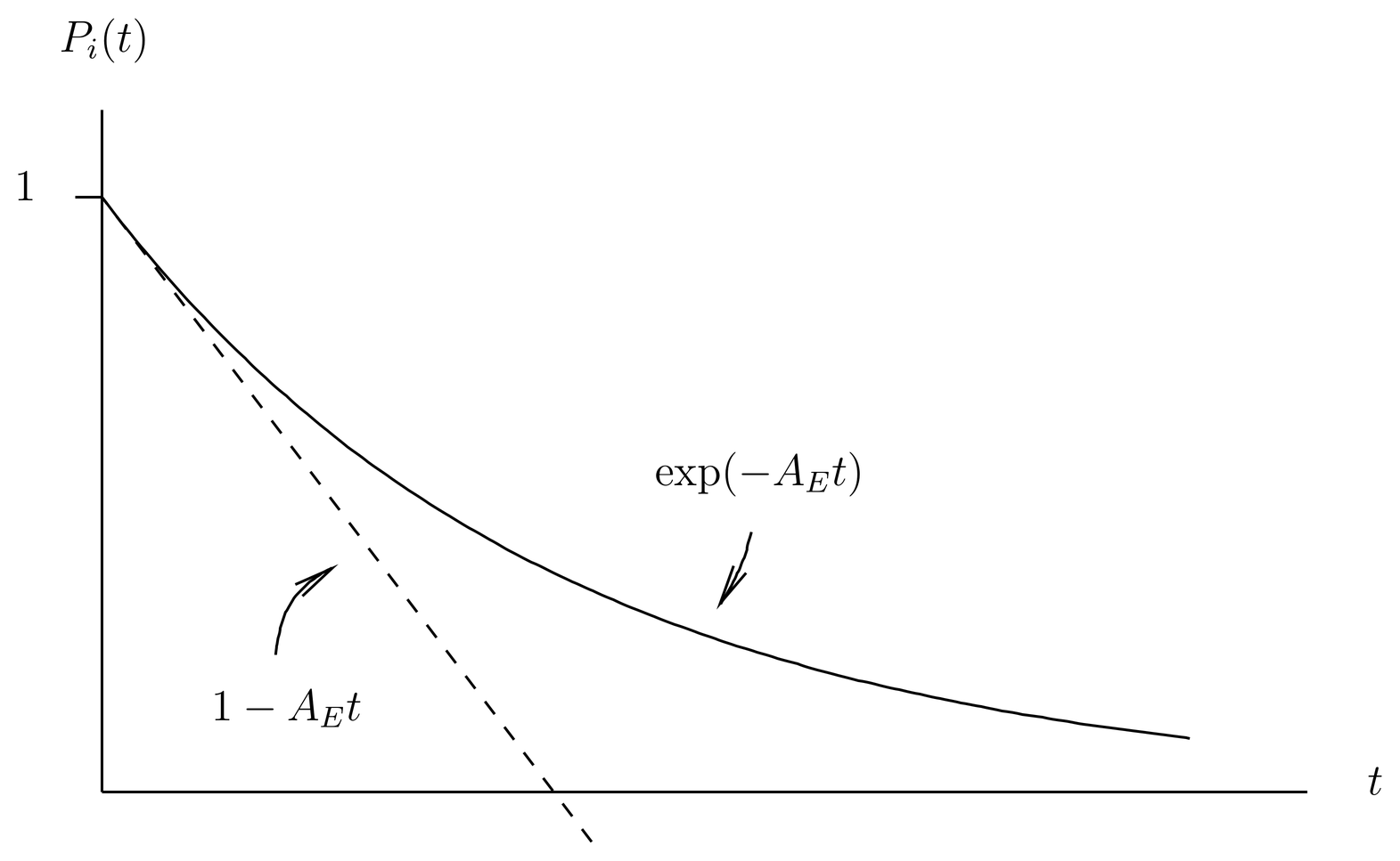
Figure 1:The prediction of first-order, time-dependent perturbation theory is that after time , the probability of remaining in the initial state goes negative. A better approximation gives an exponential decay, but this requires a different theory, valid for longer times than we have considered.
But this implies that the probability goes negative for times , as illustrated by the dotted line in Figure 1, so there must be something wrong with our theory at such long times. Therefore our theory can be valid only for times such that
measured in atomic units. Physically, must be large compared to an orbital period and small compared to the lifetime of the excited state. As we will see in Order of Magnitude of Different Multipoles, is of order in atomic units for electric dipole transitions in hydrogen, and even smaller for other types. Thus there is plenty of room for the condition (27) on to be met. (In other systems or circumstances the conditions may not be so favorable.)
Our theory breaks down for times comparable to because our calculation of the transition probability in 34. Time-Dependent Perturbation Theory{} did not take into account the depletion of probability from the initial state. To deal with the behavior atomic systems on a time scale comparable to or larger than , more powerful techniques must be used than time-dependent perturbation theory. We will see the need for this later when we take up resonance fluorescence.
Absorption of Radiation by Matter
Next we consider the process of absorption, in which the atom is initially in the lower state , from which it absorbs a photon from the field and gets lifted into the higher state (both assumed to be discrete). Since the field must contain some photons if one is to be absorbed, we assume the initial state of the field is given by , for some given list of occupation numbers . The atom can absorb a photon from any mode that initially has photons in it (but for long times, only those that nearly conserve energy will be important), so the state of the system after some time will be a linear combination of final states in which one of the modes has one fewer photon than in the initial state. In the following calculation, we let stand for the mode from which a photon has been absorbed, so that effectively also becomes a label of final states. That is, we take our initial and final states to be
where it is understood that all occupations numbers are identical in the initial and final states except in mode . The resonance frequency we will use is
which is the same as the one we had for spontaneous emission except for the sign.
Now the matrix element has the form
where again the general structure of and is indicated by (15). We see now that the only term from the sum in (15) that survives the field scalar product is the annihilation operator for , because this is the only operator that will lower the number of photons in mode by one. Furthermore, we have
so after the field scalar product is taken, we are left with
The atomic matrix element is the same as in the process of emission, except it is complex conjugated. Finally, when we use this matrix element to compute the transition rate, we have
This would be fine if we had exact knowledge of the initial state of the electromagnetic field (if we knew it was in the pure state , and if we knew exactly what all the were), but in practice we often do not have such information. Often we have only statistical information about the initial state of the field; this is certainly true for black body radiation, but it is also usually true for other types of radiation fields, including laser light. Let us suppose, therefore, that we only know some probability distribution for the occupation numbers, say, , which is the probability for a specific list of occupation numbers. For example, in thermal equilibrium (black body radiation), we would have
Working with such a probability distribution is equivalent to working with a density operator for the electromagnetic field that is diagonal in the occupation number representation,
As explained in 03. The Density Operator, the absence of off-diagonal terms means that the relative phases between different occupation number states are random.
Under such a statistical assumption, we should replace by its average over the probability distribution. This involves placing a sum over times before the right hand side of (34). But the only term in the right hand side that depends on is the single factor of itself, which then gets replaced by its average,
Finally, we can replace the sum on by the usual limit as ,
where we sum over all states (the modes from which the photon could be absorbed) because we are only interested here in the total rate of absorption. As usual, the -integral is trivial because of the -function. We obtain
Absorption of Isotropic and Unpolarized Radiation
The average number of photons per mode is a function of , that is, in general it depends on , , and . But if the radiation is isotropic and unpolarized, then by definition depends only on the magnitude of the wave vector (or equivalently, on the frequency ). For simplicity, let us consider this case. Then can be taken out of the sum and integral in (39), and what remains is the average of the squared matrix element, as in (24). The result is
which is the rate of absorption for isotropic, unpolarized radiation. It is just times the Einstein -coefficient, a simple result.
It is, however, more convenient to express in terms of macroscopic quantities. The average number of photons in mode can be expressed macroscopically in terms of the energy density per unit frequency interval. This follows from writing out the energy density (energy per unit volume) of the field in a box,
where the limit is indicated. But if the radiation is unpolarized and isotropic, then the entire summand/integrand becomes independent of and , and can be replaced by . This gives
where it is understood that is a function only of . But this is equivalent to
This is really an elementary result, which just amounts to counting states. Of course, if we use (39) for , we obtain the usual Planck formula for .
Equations~(40) and (43) show that the rate of absorption is proportional to . Following Einstein, we write this relationship in the form
which serves to define , the Einstein -coefficient. Now (40), (43) and (44) can be used to obtain a relation between the Einstein - and -coefficients,
The relation between the Einstein and coefficients depends only on the counting of states in the electromagnetic field; it does not depend on the nature of the matter interacting with the radiation. Thus, (45) is valid for radiation interacting with any kind of matter (atoms in a gas, nuclei inside a star, etc). (45) is of use in the semiclassical theory of radiation, in which can be computed after a tricky and convoluted calculation, but is impossible.
Stimulated Emission
Finally, let us examine the process of emission in the presence of radiation. This is just like the spontaneous emission considered above, except the photon field is not assumed to be empty in the initial state. We let the initial and final states be
where it is understood that all occupation numbers are the same in the initial and final states, except in mode , which gains a photon. Now the matrix element for time-dependent perturbation theory has the form
and only the creation operator for survives in the sum (15). Also, we have
so that when we compute the transition rate, we obtain
which is exactly the same as the absorption rate (34) except for the replacement of by . It is also the same as the rate of spontaneous emission (20), except for the replacement of 1 by . Thus, the part is regarded as the rate of stimulated emission, and the 1 part is the rate of spontaneous emission.
If the sum on is taken over all photon states, then the result is the total rate of emission of the photon into any final state. Of course energy conservation restricts which final states the photon may go into, and the matrix element has a dependence on the direction of the outgoing photon, but there are still many possible final states. But because of the numerator in , those states that are already populated by photons are more likely to receive the emitted photon. In this way, photon states that are already populated tend to become more populated; one can say that bosons not only can occupy the same state, they like to occupy the same state. The classical or semiclassical interpretation of this process is simple, for if we imagine an initial photon state that is already populated as a classical electromagnetic wave, assumed to be in resonance with the atomic transition, then the wave shakes the atom at its resonant frequency and stimulates the emission of a new photon with the same frequency, wave vector and polarization as the wave itself.
This is the basic principle of amplification in lasers and masers, which typically work by passing radiation through a cavity containing a population of atoms in an excited state. These atoms are stimulated to emit photons into one or a few states, which tends to increase the amplitude of the wave. However, stimulated emission is in competition with absorption, which according to (34) has a transition rate that is also proportional to . Of course, absorption removes photons from the wave. Therefore lasing normally requires a population inversion, to give the advantage to the process of emission.
The +1 in (48), representing the rate of spontaneous emission, is generally parasitic to laser operation, since the emitted photon is just as happy to go out in any direction or polarization. For proper laser operation, the population inversion must be sufficiently favorable to overcome these and other losses.
Let us now assume that the initial radiation field is represented by an isotropic and unpolarized ensemble , just as we did for absorption. Then we can average over the ensemble and sum over modes in (49), to obtain
We see that the rate of stimulated emission is equal to the rate of absorption; this is called detailed balance, which means that transition rates between two microscopic states are equal. Detailed balance is not necessary to establish thermal equilibrium, but it generally holds in first order perturbation theory, due to the Hermiticity of the perturbing Hamiltonian .
Decomposition of into Multipoles
We will now analyze the atomic matrix element , given by (18), which applies to both emission and absorption. First we note that the phase in the exponent in (18) is small over the size of the atom. This follows easily in atomic units, in which the size of the atom is , and the frequency of the emitted or absorbed radiation is . But since in atomic units, and since , we have
If is not too large, this is a small quantity. Similarly, we find that the term in (18) is of order relative to . Therefore expanding in powers of is equivalent to expanding in powers of . We write
for this expansion, where
As we shall show, the term is the electric dipole () term, while the term contains both the magnetic dipole () term and the electric quadrupole () term.
First we work on . We invoke the following commutator, which is equivalent to the Heisenberg equations of motion for the operator ,
Here can be taken to be the unperturbed atomic Hamiltonian seen in (8) since the field Hamiltonian will not contribute. Using (55) in (53), we find
where . The matrix element of is proportional to the matrix element of the electric dipole operator, defined by
so we will henceforth refer to as the electric dipole contribution to the matrix element. We will write this contribution as
Because the electric dipole term is the leading term in the expansion in , the assumption is sometimes called the electric dipole approximation.
As for , we work on the orbital part first [the second term in (54)]. We note that the two factors in this term can be written in any order, since
because the light waves are transverse. We use the summation convention and break this term up into its symmetric and antisymmetric parts, finding,
The antisymmetric part can be written in terms of the orbital angular momentum,
which, when combined with the spin part of [the first term in (54)], gives the magnetic dipole contribution to the matrix element,
With the help of the commutation relations (55) and (60), the symmetric part of can be transformed as follows:
where we have swapped and in the second term of the first expression. In the final expression it is customary to replace the operator by , where is the electric quadrupole operator,
Quadrupole moments were discussed in The Multipole Expansion in Electrostatics; see (89). The extra term proportional to in (67) makes no contribution to the matrix element (66) because . We include it anyway because it makes the tensor a irreducible tensor operator. The extra term in (67) has the effect of subtracting off the component of the tensor product . Altogether, we find the electric quadrupole contribution to the matrix element,
In these operations on the atomic matrix element , we have been doing two things: one is to expand the matrix element in the small quantity , and the other is to organize the results into irreducible tensor operators. We have done this in an ad hoc manner for the first three terms (, and ) of the multipole expansion; these are the terms that are usually of most importance in atomic physics. However, in nuclear and molecular physics, one often has need to go to higher order in the multipole expansion, and one must be more systematic.
It is not necessary to expand in powers of in order to carry out the multipole expansion, and in some applications is not small. This is notably true in nuclear physics, where is not as favorable as in atomic applications. To carry out the multipole expansion without expanding in powers of , it is convenient to organize the photon states as eigenfunctions of ), rather than as eigenfunctions of as we have done. The eigenfunctions of are known as vector spherical harmonics; they are a generalization of the ordinary spherical harmonics to vector fields. The theory of the vector spherical harmonics is essentially a straightforward application of rotation operators to the wave functions of a spin-1 particle, but it is sufficiently lengthy that we will not go into it in detail.
However, we remark that if is small, it means that the phase of the light wave is nearly constant over the spatial extent of the radiator, namely, the atom. We recall that in scattering theory we have -wave scattering in the long wavelength limit, because the radiators stimulated by the incident wave are all in phase. In -wave scattering, the scattered wave is isotropic and the cross is independent of angle. In the case of a scalar wave, it is possible to radiate -waves, but for transverse vector waves such as electromagnetic waves there are no -waves. Instead, the lowest angular momentum state for the radiated waves is the state, which comes in two varieties, odd and even parity, representing electric and magnetic dipole radiation. These give the simplest radiation patterns possible with electromagnetic waves. If is not small, it means that it is necessary to take into account the phase differences in the radiated wave across the radiator, which can be regarded as the effects of retardation.
Order of Magnitude of Different Multipoles
The total matrix element is a sum of terms in the multipole expansion, but if is small, there will be one term of leading order that dominates the others. Thus, in atomic transitions, the radiation is dominantly of one type (, , etc.), although higher order corrections are present, in general. The transition rate for the different multipole types is conveniently estimated by working in atomic units and expressing the dependence of on and the fine structure constant . For simplicity, we will ignore the dependence on the atomic quantum numbers, but if any of these are large, they should be taken into account, too. Then we find that the matrix element of (59) is of order in atomic units, while the matrix elements and , given by (64) and (68), are both of order . Therefore the spontaneous transition rate, given by (25), goes as for transitions, and as for and transitions. We see that if is not too large, the condition (27) on time scales is easily met. In fact, for and for quantum numbers of order unity, the lifetimes for electric dipole transitions are of the order of times smaller than the orbital period of the electron. For example, in the transition in hydrogen (the fastest one), we can think of the electron as orbiting on the order of a million times before dropping into the ground state. The factor becomes for and transitions that are even slower.
Selection Rules
The operators that occur in the various multipole matrix elements (59), (64), and (68), can be expressed in terms of irreducible tensor operators . These operators also have well defined transformation properties under conjugation by parity . Table~radnmatt-1 summarizes the different operators we have considered and lists their values and parities. The general rules are that an or an operator is an irreducible tensor operator (perhaps in Cartesian form) of order , and that an -operator has parity and an -operator has parity .
Table 1:Multipole terms in the expansion of the transition matrix element. The order and parity of the irreducible tensor operator are tabulated. \par
| Selection Rules | ||||
|---|---|---|---|---|
| r | 1 | |||
| 1 | ||||
| 2 |
These operators are sandwiched between atomic states and , which are eigenstates of various angular momentum operators and also of parity (ignoring the weak interactions). The Wigner-Eckart theorem and rules of parity can be applied to the resulting matrix elements to obtain selection rules. For example, consider a model of hydrogen in which we include the fine structure corrections but ignore the hyperfine structure. Let us denote the upper state by and the lower state by , so the different multipole contributions have the form . The selection rules for transitions are familiar; the operator is a irreducible tensor operator both under total rotations, generated by , and under purely orbital rotations, generated by . Therefore the Wigner-Eckart theorem gives the selection rules and ; but the case is excluded by parity (otherwise known as Laporte’s rule). For transitions, the operator is a irreducible tensor operator under total rotations, generated by , but is the sum of a and a operator under purely spatial rotations. Again, the Wigner-Eckart theorem gives and , but this time parity excludes the case . Similarly, for transitions, the case , which would be allowed by the Wigner-Eckart theorem, is excluded by parity. These rules are summarized in Table~radnmatt-1.
There are further restrictions imposed by the Wigner-Eckart theorem. For example, an transition is not allowed, because it is impossible to reach from . Similarly, is impossible in transitions. In hydrogen, only half-integral are allowed, but in atoms with an even number of electrons, is integral, and there are further rules of a similar sort. For example, is impossible in either or transitions.
An interesting case in hydrogen is the transition. Of course, the states can make an transition to the ground state, and do so with a lifetime on the order of 10-9~sec. However, the is forbidden as an transition, because of parity. It would appear from Table~radnmatt-1 that this transition is allowed as an transition, but it turns out that the matrix element (64) vanishes because of the orthogonality of the radial wave functions. In detail, the story of the transition in this case is somewhat complicated. It turns out that if the hydrogen atom is modeled with the Dirac equation, then the matrix element does not exactly vanish, but it is higher order in powers of than one would normally expect, and is very small. A similar result is obtained with the Schr"odinger-Pauli theory, if we expand to higher order in and extract the contribution from some higher order terms (although the Schr"odinger-Pauli theory is not reliable for terms that are higher order in ). Suffice it to say that the matrix element is very small. What about higher multipole moments in the transition? The transition is forbidden in this case because it would be both a and an transition. Similarly, we can see that all higher order multipole transitions are forbidden, because we cannot reach from , when . In fact, it turns out that the principal decay mode of the metastable state is a two-photon decay to the state, with a lifetime of about 10-1~sec. See Prob. Paragraph.
Speaking of small effects, we may also notice that the can decay to the state by an transition, since the latter is lower in energy by the (small) Lamb shift. But this rate is much smaller than the two-photon decay mentioned above, and does not contribute much to the overall decay rate. This transition is, however, important when driven by microwaves at or near the resonant frequency of 1.06 GHz. Indeed, Lamb and Retherford first used such microwave techniques in 1949 to make an unequivocal and high precision measurement of the Lamb shift.
Angle and Polarization Dependence of Radiation
Let us return now to the process of spontaneous emission, and consider the intensity of the emitted radiation as a function of angle and polarization. We will work this out only for electric dipole radiation, the most common case. We can imagine an experimental situation such as that illustrated in Figure 2, which effectively measures the polarization and direction of the outgoing photon. In the following we will assume for simplicity that some state () of circular polarization is measured, but other states of polarization are only slightly more complicated to analyze.
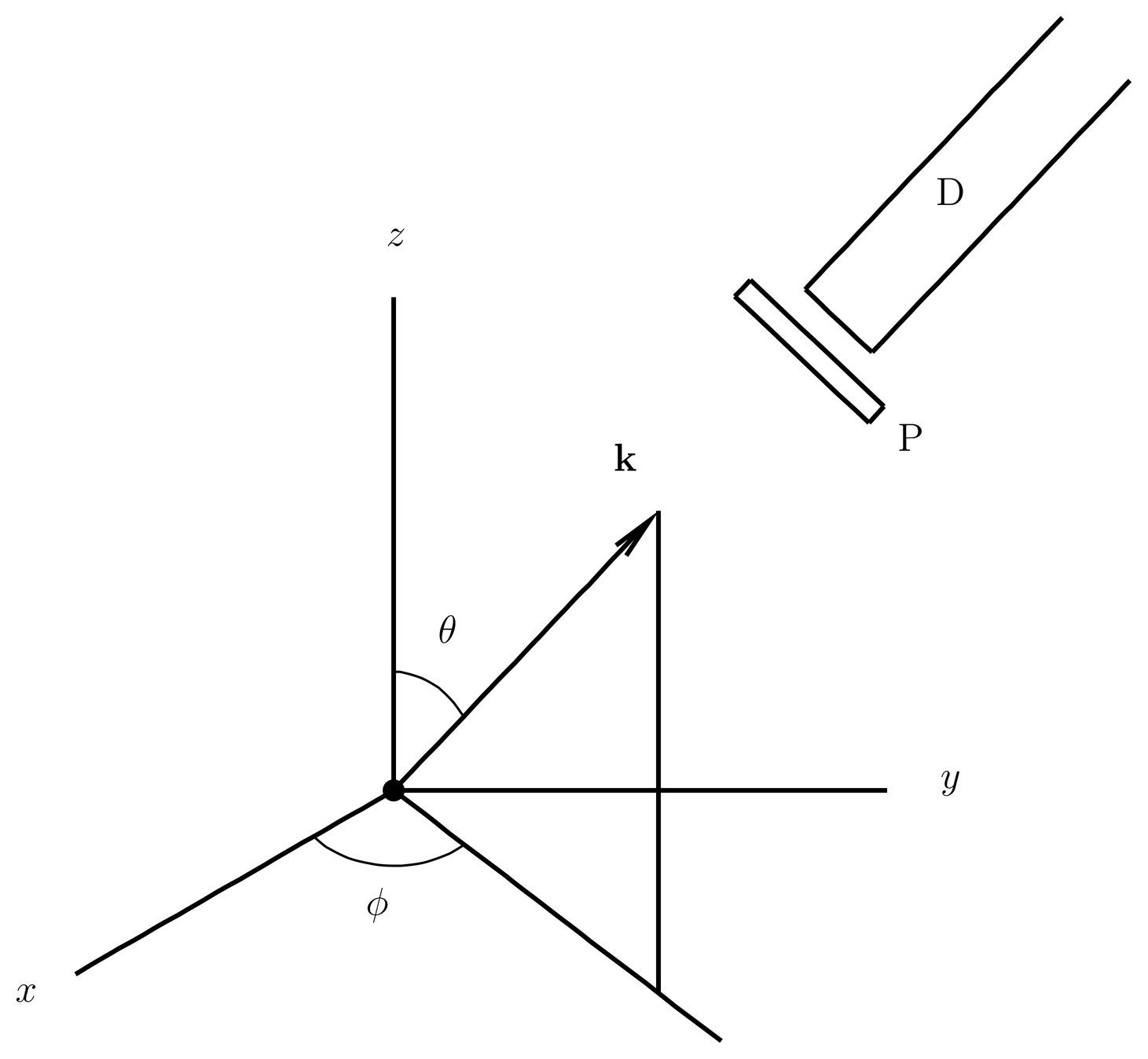
Figure 2:Photons are emitted from a source of excited atoms at the origin of the coordinates. Photons emitted in a small solid angle around the direction are filtered by the polarizer , which passes only one state of polarization, and are detected by the detector .
We start with (23), into which we substitute (57) for the electric dipole approximation to the matrix element. This gives
where , and where
For simplicity we assume the atom is a hydrogen-like atom in the fine-structure model (we ignore hyperfine effects, etc.), and we take the upper and lower states to be and , as above, so that
(However, hardly anything changes if we use the eigenstates of a multi-electron atom.)
It is convenient to expand in terms of the spherical basis as in (6),
because then the components are components of a rank~1 irreducible tensor operator. We also use (80) to express in terms of the spherical basis. Then we have
where is defined by (78) and is the corresponding -matrix, and where we use (32).
Now when we compute , we obtain a sum over the matrix elements of , which can be transformed by the Wigner-Eckart theorem [see (51)]:
But by the selection rule (56) for the Clebsch-Gordan coefficients, only the term survives in the sum. Therefore when we combine all the pieces together, we obtain the following expression for the differential transition rate for electric dipole transitions:
where now it is understood that ( is not summed over). This is a convenient expression, because the reduced matrix element shows the dependence of the transition rate on the manifolds and of the initial and final states, the Clebsch-Gordan coefficient shows the dependence on the magnetic quantum numbers, and the -matrix shows the dependence on the polarization and direction of the outgoing photon. Furthermore, writing the -matrix in Euler angle form and using (69), we have
where as illustrated in Figure 2 are the spherical angles of and where we suppress all leading factors and concentrate on the dependence on and . We see that the intensity of the emitted radiation is independent of the azimuthal angle , as we would expect since the initial and final states are eigenstates of . Finally, we can invoke (72) for the reduced rotation matrix to determine the angular distribution as a function of for different choices of and . The angular distribution is plotted in Figure 3 for different cases. By the way, the quantity has a simple interpretation, for if we write its definition in the form , we see that is just the quantum number of the emitted photon, since the total of the combined matter-field system is conserved in the emission process.
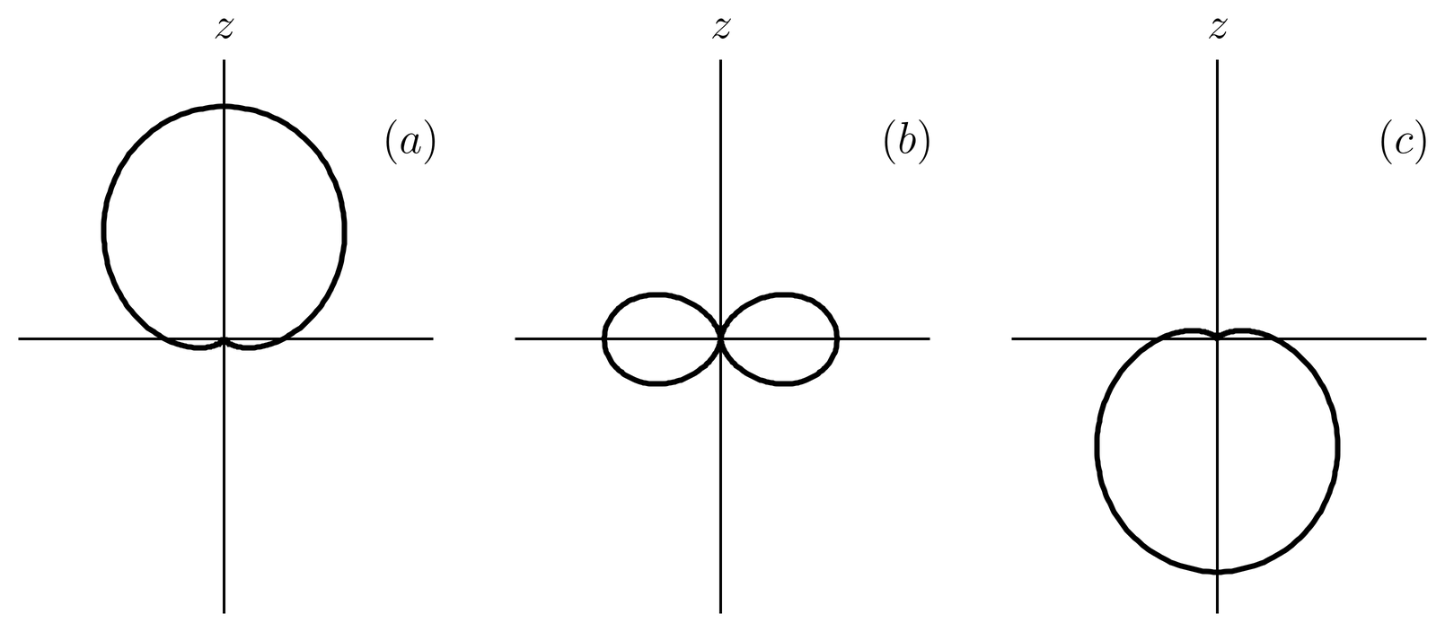
Figure 3:Polar plots of intensity of electric dipole radiation for different cases. Case , ; case , , ; case , . Intensity is azimuthally symmetric.
The radiation patterns in Figure 2 can be seen experimentally by placing the source (for example, a gas discharge tube) in a strong magnetic field, which will split the various magnetic substates of the otherwise degenerate initial and final states, so that a transition with a definite value of can be observed. On the other hand, in many practical circumstances there is no magnetic field to split these substates, nor is the initial ensemble of atoms polarized. In such cases, the atom has an equal probability of being in any of the magnetic substates of the initial, degenerate atomic level; and all transitions to the various magnetic substates of the final, degenerate atomic level lie on top of one another (they have the same frequency), so the spectroscope simply sees a single line whose intensity is the superposition of the intensities of possibly several transitions. Furthermore, if the initial state of the atom is unpolarized, then it has no preferred direction, and the emitted radiation is isotropic. In this case we might as well ask for the total transition rate (integrated over all solid angles and summed over polarizations). We will now analyze this case for electric dipole radiation.
The Total Transition Rate
We begin by computing the total transition rate. We could do this by integrating (76) over solid angles and summing it over polarizations, but it is just as easy to go back to (25), and to use the electric dipole expression (57) for the matrix element. Also, for simplicity, we will use the simple electrostatic, spinless model for the states of the one-electron atom, that is, we will ignore the fine structure corrections. Then combining (24) and (57), we have
where now
Here the initial and final states are and , respectively. The polarization sum in (78) is easy if we use the completeness relation (63) for the polarization vectors. This gives
Next, the angular integration of this over is easy, since the first term is independent of angle and the second term is just the angle average of one component of a vector. Thus we have
Altogether, (78) becomes
As for the , it is convenient to use it in complex conjugated form,
where
We expand in this expression in the spherical basis as in (72), so that
and so that
But by (18), the quantity can be expressed in terms of , where are the spherical angles in -space. This causes the matrix element in (86) to factor into a radial part times an angular part,
where
and
We apply the 3- formula (83) to the latter, to obtain
Then (86) becomes
which shows how the total transition rate depends on the magnetic quantum numbers of the transition.
Now, however, we assume that the initial state is unpolarized and that we don’t care which final state the atom falls into. Then we obtain an effective value of by averaging over initial magnetic substates, and summing over final magnetic substates. This causes the replacement,
But when we use (91) in this, the and sums can be done,
where we use the orthonormality relation (54) of the Clebsch-Gordan coefficients. Finally, putting all the pieces together and using (25), we find the effective Einstein -coefficient for electric dipole radiation,
A standard reference for the material in these notes is Bethe and Salpeter, Quantum Mechanics of One- and Two-Electron Atoms, which includes tables of dipole transition rates.
Problems
Problem 1.
The perturbation expansion (\eqr\cn.6) is valid if . Compute the energy flux (in watts per square cm) of light for which the rms electric field of the light wave is equal to the electric field strength due to the proton in a hydrogen atom at the Bohr radius. There is current experimental interest in the physics that arises at such high fields. The fields are created by focussing laser light onto a small region.
Problem 2.
Compute the lifetime of the 21~cm transition in Hydrogen, . Here is the total angular momentum , orbital plus spin for the electron plus spin for the proton. The splitting between the energy levels is given by Eq.~(\eqr\hyperfine.50), where is the proton -factor, and are the nuclear and Bohr magnetons, respectively, and is the Bohr radius. Assume the upper state is unpolarized (equal probabilities of being in the different magnetic substates). The lifetime is the inverse of the Einstein coefficient. This lifetime determines the radio power radiated by galactic clouds of atomic hydrogen.
Problem 3.
A hydrogen atom is at distance from a hot blue star with radius and surface temperature , which radiates significantly in the ultraviolet. Assume , so that the light coming from the star is concentrated in a narrow range of solid angles. Assume the surface of the star radiates as a blackbody. Assume the atom is unpolarized. When the atom absorbs a photon, taking it from the state to the state, it absorbs the photon momentum and suffers a recoil; then in short order ( sec), it reemits a photon and drops back into the ground state. But since the reemission of the photon is isotropic (for an unpolarized atom), the average momentum transferred by the emitted photon is zero. In this way, the atom feels an effective force because of the absorption of photons from the star. Find an expression for this force in terms of , , , and other appropriate parameters. Ignore all atomic states except the and .
Problem 4.
The matter Hamiltonian (\eqr\cn.5) is not a special case of the Hamiltonian (\eqr\cn.3), because the potential in (\eqr\cn.5) is an external, -number potential introduced in an {\it ad hoc} manner to describe the interaction of the atomic electron with the nucleus, assumed to be infinitely massive and situated at the origin of the coordinates. It is certainly plausible that (\eqr\cn.5) should represent the dynamics of the atomic electron interacting with the electrostatic field of the nucleus and with the quantized electromagnetic field, but it would be nice to actually derive (\eqr\cn.5) from (\eqr\cn.3), taking into account both the dynamics of the electron and that of the nucleus.
(a) Consider a two-particle system with masses } and and charges and . This covers the case of hydrogen, for which , and positronium (a bound state of an electron and a positron), for which . Write the matter Hamiltonian as
where we ignore the terms because we will be working only to the accuracy of the or electric dipole approximation. In this approximation, is of order and is negligible, where is the separation between the two particles. This means that or can be approximated by , where is the center of mass position.
Perform a transformation from the particle positions (,) and momenta (,) to center-of-mass positions and momenta (,) and relative positions and momenta (,), as in Two-Body Central Force Motion. Let be the total mass of the system and the reduced mass, as in Two-Body Central Force Motion. Show that in the dipole approximation, the Hamiltonian (95) can be transformed into
(b) This is similar to the Hamiltonian (5). Differences include the center-of-mass kinetic energy term , present here but absent in (5); the replacement of in (5) by here; and the fact that the Hilbert space contains the center-of-mass degrees of freedom as well as those of the electron and the electromagntic field. Write the total Hamiltonian (matter plus field) in the form
where
Write the eigenstates of as a product of a matter times a field part, where the matter eigenstate has the form , where refers to an atomic state and is an eigenstate of the center-of-mass Hamiltonian (with ). Notice that there three classes of degrees of freedom now, the relative coordinates in the atom, the center of mass coordinates, and the field.
Assume the system is initially in the excited atomic state with no photons in the field, as in Spontaneous Emission, and with the initial center of mass momentum . Use first-order time-dependent perturbation theory to compute the differential transition rate as in (23), with replaced by the electric dipole approximation as in (53). You want the rate at which photons make transitions into a small cone, but you do not care about the center of mass momentum, so you should sum over all values of in the final state.
Show that in addition to the physics discussed in Secs.~Spontaneous Emission and Decomposition of into Multipoles, we find the fact that the atom as a whole recoils upon the emission of the photon. The photon frequency is no longer , but rather there is a correction, which is small since . Compute this correction as a function of to first order in small quantities. This correction is the Doppler shift due to the recoil of the atom. It is certainly small, but important in some applications, for example, in laser cooling of atomic gases and in the M"ossbauer effect (see The Nucleus and the M"ossbauer Effect).