24. The Stark Effect in Hydrogen and Alkali Atoms
Introduction
In these notes we consider the Stark effect in hydrogen and alkali atoms as a physically interesting example of bound state perturbation theory. The Stark effect concerns the behavior of atoms in external electric fields. We choose hydrogen and alkali atoms because they are single-electron atoms (in the case of alkalis, this is a model). We particularly emphasize the role that symmetry principles play in the analysis of the Stark effect, and the physical ramifications.
The first observations of the splitting of spectral lines by electric fields were made by Stark in 1913, for which he was awarded the Nobel prize in 1919. Stark was an early supporter of Einstein’s relativity theory, as well as Einstein’s ideas about photons, about which most physicists of the time were very skeptical. After the Nazis came to power, however, he obtained a high position in the scientific establishment and, along with fellow Nobel laureate Philipp Lenard, promoted the notion that “Jewish physics,” which meant especially the theory of relativity, was degenerate and false. He also attacked Heisenberg, who defended both Einstein and relativity. After World War II, he was sentenced to four years in prison by a denazification court. Today Stark is remembered probably more for his racist and nationalistic political views than for his science.
Atomic Models
The one-electron atom will be modeled with the central force Hamiltonian,
For hydrogen the potential is
while for the alkalis the potential is described in Central Force Model of Alkali Atoms.
In this Hamiltonian we ignore spin and other small effects such as relativistic corrections, hyperfine effects and the Lamb shift. These effects cause a splitting and shifting of the energy levels of our simplified model, as well as the introduction of new quantum numbers and new degrees of freedom. But these effects are all small, and if the applied electric field is strong enough, it will overwhelm them and the physical consequences will be much as we shall describe them with our simplified model. For weak applied electric fields, however, a realistic treatment would require that all the small effects (the external electric field included) be treated together. See Prob.~\prbrstark-2, in which the transition from weak to strong electric fields is explored.
The Unperturbed System
Before embarking on perturbation theory, we must understand the unperturbed system, its energies, eigenstates and their degeneracies. In the electrostatic model, the unperturbed energy levels in hydrogen are
Table 1). Here we ignore the small difference between the electron mass and the reduced mass . According to (24), these levels are -fold degenerate. In the case of the alkalis, the energy levels have the form , and are -fold degenerate. There is no simple formula for the alkali levels , but for given , the energies are an increasing function of , as shown in case of sodium in Fig.~\figr\hydrogen.3. As we shall see, the differences in the degeneracies has an important impact on the Stark effect in hydrogen as compared to that in the alkalis. As explained in 17. Hydrogen and Hydrogen-Like Atoms, the extra degeneracy in hydrogen is due to the extra symmetry [ instead of ] that it possesses, in comparison with a generic central force problem, such as an alkali in the model described in Central Force Model of Alkali Atoms. As for the eigenstates, in both hydrogen and the alkalis they have the form ; these are central force eigenfunctions of the form
Potentials and Nonperturbative Considerations
As for the perturbation, let us write for the external electric field (instead of , to avoid confusion with the energy ), and let us take it to lie in the -direction,
Thus, the perturbing potential has the form
where we set for the electron. The unperturbed potential depends on , but the perturbing potential depends on , so the perturbation breaks the full rotational symmetry of the unperturbed problem. However, the perturbed Hamiltonian is still invariant under rotations about the -axis.
Figure 1 is a plot of the total potential along the -axis, which reveals several qualitative features of the exact solution. For small , the attractive Coulomb field dominates the total potential, and we have the usual Coulomb well that supports atomic bound states. We assume the applied electric field is small compared to the electric field due to the nucleus in this region, which justifies the use of perturbation theory. This is reasonable for most realistic, laboratory strength fields , since the electric field due to the nucleus at a typical atomic distance is of the order of 109 Volts/cm. In practice, large electric fields can be created in capacitors in which the dielectric layer is very thin, for example, a layer of metal oxide, which may be only a few atoms thick. Elsewhere laboratory electric fields tend to be much weaker than those inside atoms.
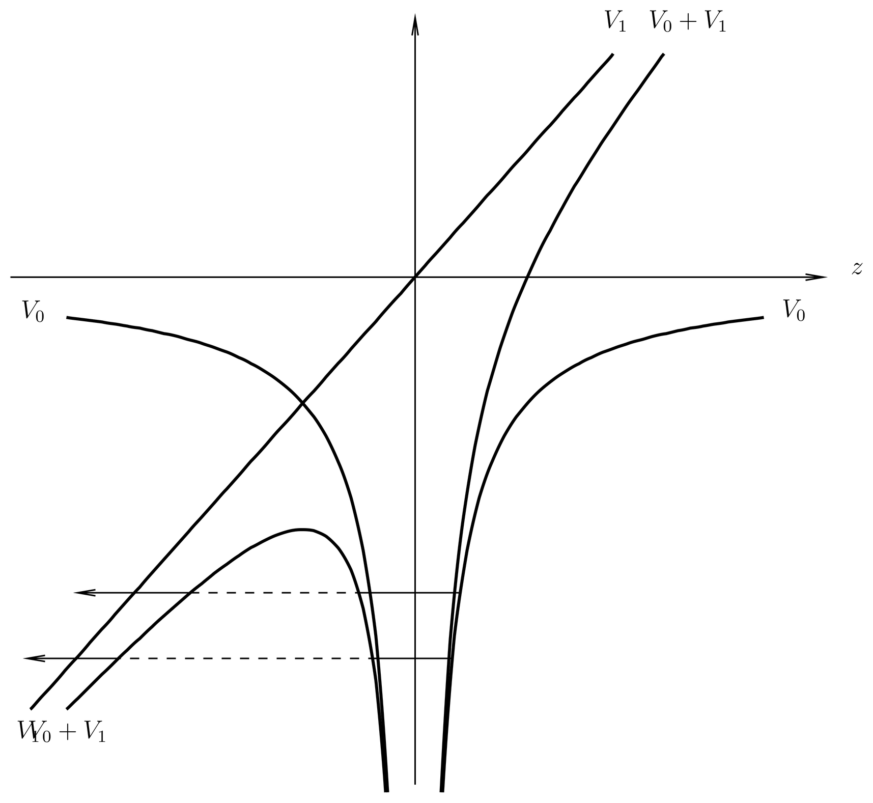
Figure 1:The total potential energy along the -axis for an atomic electron in the Stark effect. The atomic states that are bound in the absence of the external field become resonances (dotted lines) when the perturbation is turned on.
However, for large negative , the unperturbed potential goes to zero, while the perturbing potential becomes large and negative. At intermediate values of negative , the competition between the two potentials gives a maximum in the total potential. The electric force on the electron, which is the negative of the slope of the potential energy curve, is zero at the maximum of the potential, so this is the point where the applied and the nuclear electric fields cancel each other. Given the relative weakness of the applied field, the maximum must occur at a distance from the nucleus that is large in comparison to the Bohr radius . Atomic states with small principal quantum numbers lie well inside this radius (hence in the region where the external electric field is much smaller than the electric field of the nucleus). The perturbation analysis we shall perform applies to these states.
The bound states of the unperturbed system are able to tunnel through the potential barrier, as indicated by the dotted lines in the figure. We see that when an external electric field is turned on, the bound states of the atom cease to be bound in the strict sense, and become resonances. This happens regardless of how weak the external field is. This is because an electron can gain an arbitrarily large amount of energy in an uniform field if we are willing to move it far enough, and this energy can be larger than the binding energy of the atom. Electrons that tunnel through the barrier and emerge into the classically allowed region at large negative will accelerate in the external field, leaving behind an ion. This is the phenomenon of field ionization.
However, the time scale for this tunneling may be very long. As we know from WKB theory, the tunneling probability is exponentially small in the tunneling action, so we expect the deeper bound states to have longer lifetimes in the external field, perhaps extremely long lifetimes. Furthermore, as the strength of the electric field is decreased, the distance the electron must tunnel increases, and the tunneling probability decreases exponentially. On the other hand, the atom has an infinite number of very weakly bound states that pile up at , and many of these will lie above the top of the barrier when the external field is turned on. In the presence of the perturbation, these states are ionized immediately.
In the following perturbation analysis, we will see no evidence of the tunneling. A resonance can be thought of as an energy level that has both a real and an imaginary part, where the imaginary part is related to the lifetime by ; as we will see, bound state perturbation theory will only give us the shift in the real parts of the energy levels under the perturbation. The imaginary parts can be computed by various means, such as WKB theory, time-dependent perturbation theory, or (in the case of hydrogen) an exact separation of the wave equation in confocal parabolic coordinates.
No Linear Stark Effect in the Ground State
For simplicity, let us begin the perturbation analysis with the ground state of the atom, so we can use nondegenerate perturbation theory. In the case of hydrogen, the ground state is the or level, and for an alkali, the ground state has the form (for example, for ). According to (26) (with a change of notation), the first order shift in the ground state energy level is given by
which vanishes because of parity. The operator is odd under parity, while the state is one of a definite parity (even), so the matrix element vanishes. The matrix elements are the same as in the theory of electric dipole radiative transitions, and follow the same selection rules (here Laporte’s rule). See Parity and Selection Rules. As we say, there is no linear Stark effect (no first order energy shift) in the ground state of hydrogen or the alkalis.
Linear Stark Effect and Permanent Electric Dipole Moments
The linear Stark effect is closely related to the permanent electric dipole moment of the corresponding quantum state. In classical electrostatics, the dipole moment vector of a charge distribution is defined by
that is, it is the charge-weighted position vector. [This is (86).] In the presence of an external electric field , the classical dipole has the energy,
which is the potential energy of orientation of the dipole.
To describe the quantum mechanics of a single charged particle, we may replace in (8) by (see Physical Significance of the Probability Density and Current), and interpret the result as the expectation value of the dipole moment operator,
where the operator itself is given by
If there is more than one charged particle we define the dipole moment operator by the sum,
A quantum state is considered to have a permanent electric dipole moment if the expectation value is nonzero. In the case of a single electron system with , the expectation value is
so that if is an energy eigenstate, then the first order energy shift due to the external field is
Compare this to (9). We see that there is a nonzero linear Stark effect in the quantum state if and only if the state possesses a nonzero permanent electric dipole moment. The linear relationship shown in (14) between the energy shift and the applied electric field explains the terminology, “linear Stark effect.”
No Linear Stark Effect in Any Nondegenerate State of Any System
Since we failed to find a linear Stark effect in the ground state of hydrogen or alkalis, let us look for one in other systems. For the time being we consider only nondegenerate energy eigenstates.
Suppose we have a Hamiltonian for any isolated system (atom, molecule, nucleus, etc., of arbitrary complexity). could be the Hamiltonian for hydrogen or the alkali atom, but with all the small corrections and (in the case of the alkali) multiparticle effects included, or it could be a multiparticle system. The 0 subscript means the unperturbed system; the system is no longer isolated after the external field is turned on. We suppose this Hamiltonian commutes with parity, . This is an extremely good approximation for most systems, since parity violations come from the weak interactions which are extremely small in most circumstances. In the following we will neglect small parity violating effects, and treat all Hamiltonians for isolated systems as if they commute with parity.
Now let be a nondegenerate energy eigenstate of such a system. It was shown in Parity and Energy Eigenstates in Isolated Systems that such eigenstates are also eigenstates of parity, that is
where . This is really a simple application of Theorem Theorem. Thus,
because only connects states of opposite parity.
The vanishing of the linear Stark effect in the ground state of hydrogen and the alkalis was not special to those systems or the models we used for them, but follows from conservation of parity and the fact that we are considering nondegenerate states.
No Linear Stark Effect in the Excited States of Alkalis
We see that if we wish to find a nonvanishing linear Stark effect, we must examine degenerate states. We begin with the excited states of the alkalis, which are simpler than the excited states of hydrogen because the degeneracy is smaller. These states have energies and are -fold degenerate, that is, they are degenerate for , so to find the first order energy shifts we must use degenerate perturbation theory. According to \pertth.6, the first order energy shifts for the Stark effect in the excited states of the alkalis are the eigenvalues of the matrix indexed by and ,
Notice that and are the same on both sides of these matrix elements, because these indices label the unperturbed, degenerate level. Only the index is allowed to be different on the two sides, because this index labels the basis kets lying in the unperturbed eigenspace.
But we need not do any work to find the eigenvalues of this matrix, because all the matrix elements (17) vanish, again by parity. This is because the parity of a central force eigenstate is (see Parity and Selection Rules), which is the same on both sides of the matrix elements (17). So once again we fail to find a linear Stark effect.
Degeneracies and Parity in Generic, Isolated Systems
To review some facts about isolated systems, the presentation of Secs. Energy Eigenstates in Isolated Systems--The Nucleus and the M"ossbauer Effect led to Theorem Theorem, which states that the energy eigenspaces of isolated systems consist of one or more irreducible subspaces under rotations. We also explained that with a few exceptions, including the electrostatic model of hydrogen, these eigenspaces consist of just a single irreducible subspace, characterized by a value of . Then, in Parity and Energy Eigenstates in Isolated Systems, we explained that in isolated systems that are invariant under parity, the energy eigenspaces consisting of a single irreducible subspace are also eigenspaces of parity, that is, they are states of a definite parity. If we call these energy levels , where is a sequencing number of the energy for a given value of , then the matrix needed to compute the first order Stark effect on energy level is
where is given by (12). But since is odd under parity (it is a true vector), and since the parities of the two states on the two sides of the matrix element (18) are the same, this matrix element vanishes. This implies the vanishing of the linear Stark effect in energy eigenstates of generic, isolated systems.
We see that to find a nonvanishing linear Stark effect in an isolated system we must find a system in which there is a degeneracy between different energy multiplets for different values of , and, moreover, we must have different multiplets of the same energy but opposite parity. The most important example where such multiplets of the same energy but opposite parity occur is the excited states of hydrogen, to which we now turn.
Linear Stark Effect in the Excited States of Hydrogen
The excited states of hydrogen () have a degeneracy between states of opposite parity, since and since the parity is even for even and odd for odd . According to first order, degenerate perturbation theory, the shifts in the energy levels are given by the eigenvalues of the matrix, indexed by and ,
Notice the indices that are primed and those that are not. This is potentially a large matrix, but many of the matrix elements vanish because of various symmetry considerations. The -selection rule, which follows from the Wigner-Eckart theorem and parity, is the same as in the theory of dipole transitions, namely, (the Wigner-Eckart theorem would allow , but this is excluded by parity). There is also a selection rule on the magnetic quantum number: since the operator is the component of a irreducible tensor operator [see (17)], the matrix element vanishes unless .
Consider, for example, the case . The four degenerate states include the level, with eigenstate , and the level, with eigenstates for . According to the selection rules, only the states and are connected by the perturbation. Therefore of the 16 matrix elements in the matrix, the only nonvanishing ones are
and its complex conjugate. This matrix element is easily evaluated by resorting to the hydrogen radial wave functions, given in The Wave Functions. The result is real and negative, so that defined above is positive. We find
The energy is of the order of the energy needed to shift the electron from one side of the atom to the other in the external field.
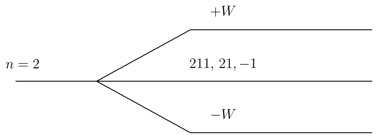
Figure 2:The Stark effect splits the level of hydrogen into three levels, of which one is two-fold degenerate.
The matrix connecting the two states and is
and its eigenvalues are the first order energy shifts in the level,
In addition, the two states and do not shift their energies at first order, so the other two eigenvalues of the matrix (19) are . The energy shifts are illustrated in Figure 2, in which the states are those with energy shifts . We see that the four-fold degeneracy of the state of hydrogen is only partially lifted at first order in the perturbation, since and remain degenerate at this order.
Explanation of Remaining Degeneracy
We may ask whether this remaining degeneracy is lifted at some higher order of perturbation theory, or whether it persists to all orders. To answer this it is best to look at the exact symmetries of the full, perturbed Hamiltonian , without doing perturbation theory at all.
The unperturbed Hamiltonian, being rotationally invariant, commutes with (all three components of angular momentum), but the perturbation is only invariant under rotations about the -axis, so it only commutes with . Likewise, the unperturbed Hamiltonian commutes with parity , but the perturbation does not, so is not a symmetry of the fully perturbed system. Finally, the unperturbed Hamiltonian is invariant under time reversal ; this symmetry is preserved by the perturbation. This takes care of the obvious symmetries of the unperturbed and perturbed systems, but not the extra symmetry of hydrogen. We will not go into this in detail, except to mention that some of the extra symmetry present in the unperturbed system persists under the perturbation, a fact that is reflected in the separability of the Schr"odinger equation for the fully perturbed system in confocal parabolic coordinates. The obvious symmetries, however, are sufficient for understanding the degeneracies of the perturbed system.
Since and commute, they possess simultaneous eigenspaces that we may denote by . We consider only the bound states, so the allowed values of are discrete, and the spectrum of contains only integers (positive, negative or zero). If , then
Now consider the state . Since and , we have
that is, maps into another state with the same energy (see Time Reversal and Energy Eigenstates) but opposite value of (see (13). If this means that both and belong to ; they could even be proportional. But if then is an eigenket of and with eigenvalues and where ; thus, there must exist an eigenspace of and with eigenvalues and , that is exists and maps into .
For the spaces and are orthogonal (since the eigenvalues of Hermitian are different), so and are linearly independent, and there is a degeneracy in the energy that crosses values. We see that in systems in which commutes with both and , the energy eigenstates for which are at least two-fold degenerate.
In a little more detail, the map induced by between and is one-to-one and onto, that is, it is invertible. We see this because , being anti-unitary, maps a set of linearly independent vectors to a set of linearly independent vectors. Since the image of under inside must fit inside , we must have . But also maps into , so we must have . Altogether, this shows that and have the same dimensionality, and thus the energy eigenstates in are paired with those of the same energy in . This is just what we see to first order in perturbation theory in Figure 2, but now we can conclude that the degeneracy between the states with is exact and persists to all orders.
The same argument applies to any system in which the Hamiltonian commutes with both and . For example, in the theory of the molecule, we are interested in the motion of an electron in the field of two protons. If we imagine the protons pinned down at locations on the -axis, then the Hamiltonian commutes with both and . Then by the previous argument, all states with are at least doublets. In reality, of course, the protons are not pinned down, but rather the molecule is free to vibrate and rotate like a dumbbell. When these effects are included, it is found that the doublets become split. This is called “-doubling,” where (not ) is the standard notation for the magnetic quantum number of the electrons about the axis of a diatomic molecule.
This argument, which we have used to prove the necessity of a degeneracy for , should not be confused with Kramer’s degeneracy, which applies whenever we have a system with an odd number of fermions. In the present calculation, we are ignoring the spin of the electrons, treating them as if they were spinless particles, so Kramer’s degeneracy does not apply.
The Perturbed Eigenfunctions
To return to the Stark effect in the levels of hydrogen, we can also work out the perturbed eigenstates. These are linear combinations of the unperturbed eigenstates, with coefficients given by the eigenvectors of the matrix (22). Explicitly, we have
The coefficients in these linear combinations are the same as the coefficients in (29). In the language of 23. Bound-State Perturbation Theory, we are determining the projection of the exact eigenstates onto the unperturbed eigenspace. This is zeroth order part of the exact eigenstates, since the part orthogonal to the unperturbed eigenspace is small. Notice that even though the perturbation is small, it has caused large (order unity) changes in the eigenstates.
The perturbed eigenstates are mixtures with equal probabilities of states of opposite parity. The phases are different for the two states , causing the charge distribution to be shifted either above or below the origin on the -axis. The energy of the state is either raised or lowered compared to the unperturbed energy, depending on whether the charge distribution has been moved with or against the external field.
The Stark Effect and Radiative Transitions
There is some interesting physics involving radiative transitions and the Stark effect on the levels of hydrogen. In the absence of an external field, the level of hydrogen has a lifetime on the order of 10-9 seconds, before the atom emits a photon and drops into the state. But the level is metastable, decaying much more slowly, mainly via two photon emission, in about 10-1 seconds. This makes it easy to create a population of mainly and states of hydrogen. For example, if we knock a population of hydrogen atoms into mixture of excited states by collisions with an electron beam, then after a short time () everything will have decayed into either the state or the metastable state.
Now the state is a linear combination of the states ,
as we easily see from (27). This applies even in the absence of an applied electric field, in which case is an energy eigenstate (a stationary state). But in the presence of an applied field, states differ in energy by , and evolve with different time-dependent phases. Let us imagine that at the system is in the state given by (28). Then the probability of finding the system in the state at a later time is
that is, the system oscillates back and forth between the and states with frequency . At least, this would be the conclusion if we could turn off the radiative transitions; as it is, however, once the system enters the state, it rapidly makes a radiative transition to the ground state. The effect of turning on the electric field is to rapidly depopulate the state, causing the emission of a burst of photons.
Induced Dipole Moment in the Ground State of Hydrogen
Let us return to the ground state of hydrogen. Although the first order Stark energy shift in this state vanishes, the first order shift in the wave function is nonzero. We see this from (28), which for the present problem is
Here is the perturbed ground state. This state has a nonzero electric dipole moment, unlike the unperturbed ground state. As we say, the ground state of hydrogen does not have any permanent electric dipole moment, but it does have an induced dipole moment in the presence of an electric field. For if we compute the expectation value of the dipole operator and carry the answer to first order in the perturbation, we find
where the polarizability is given by
The - and -components vanish in (31), and is positive in (32) because the energy denominator is negative. We see that in first order perturbation theory there is a linear relationship between the dipole moment of the atom and the applied electric field. The polarizability is a scalar for the ground state of hydrogen, but more generally (for example, for molecules) it is a tensor that specifies the linear relationship between and ,
Given the polarizability of a single atom, one can compute the dielectric constant of a gas of the atoms, although for hydrogen under normal circumstances it is unrealistic to speak of a gas of atoms (as opposed to molecules). The calculation is easiest for a dilute gas; at higher densities, one must distinguish between the electric field seen by an individual atom or molecule and the macroscopic, average electric field. A good approximation at intermediate densities is afforded by the Clausius-Mossotti equation. This is an example of how electric susceptibilities can be computed from first principles.
Quadratic Stark Effect in Hydrogen
Since the first order energy shift in the ground state vanishes, it is of interest to compute the second order shift. We invoke (27) with necessary changes of notation, to write
We see that the second order energy shift can be expressed in terms of the polarizability. Because the energy shift is proportional to the square of the applied electric field, we speak of the quadratic Stark effect. This energy can also be written,
The presence of the in this formula may be puzzling, since we are accustomed to thinking of the energy of a dipole in a field as . The reason for this factor is that the dipole moment is induced by the external field, and is itself proportional to ; the energy (35) is the work done on the atom by the external field as it builds up from zero to its maximum value. The usual expression is the potential energy of orientation of a dipole of fixed strength in a fixed electric field.
It is of interest to evaluate the sum (32), to obtain a closed form expression for the polarizability . This sum contains an infinite number of terms, and, in fact, it is more complicated than it appears, because the continuum states must also be included (there is an integral over the continuum states as well as a sum over the discrete, bound states). There are various exact methods of evaluating this sum, but we will content ourselves with an estimate. We begin with the fact that the energy levels increase with , so that
But this implies that
We excluded the term in (32), but we can restore it in (37) after taking out the constant denominator, since this term vanishes anyway. The result contains a resolution of the identity, so that the sum in (37) becomes the matrix element,
This gives the estimate
An exact treatment of the sum (32) gives the result,
so the exact expression for the second order energy shift is
This energy shift is of the order of the energy of the external field contained in the volume of the atom.
The Case of Nearly Degenerate States
Let us return to the case of a generic, isolated system. As discussed previously the energy multiplets for different values of do not coincide, so there is no degeneracy between states of opposite parity, and hence, rigorously speaking, no linear Stark effect. But energy multiplets with different can come very close to one another, a seen for example in the and classes of states of sodium in Fig.~\figr\hydrogen.3, which each have an infinite number of states piling up at the continuum limit . If the energy difference between multiplets of opposite parity is very small, it is logical on physical grounds that it would not make any difference, and the system should behave as if there were a degeneracy between states of opposite parity. That is, a linear Stark effect should exist.
As for the special case of hydrogen, the exact degeneracy between the and states is only a feature of the approximation of the spinless, nonrelativistic, electrostatic model (1). In real hydrogen, the states are split into the and states, neither of which coincides exactly in energy with the state (properly, the state). The splitting between the and the states is particularly interesting; it is due to the interaction of the atomic electron with the quantized electromagnetic field, and is called the Lamb shift. Because of the Lamb shift, the state actually lies approximately 1.058 GHz above the state.
Thus, in a realistic treatment of hydrogen, there is no degeneracy between states of opposite parity, although the and levels come very close. Therefore there is, rigorously speaking, no linear Stark effect in the levels of hydrogen either, and the dependence of the energy shift on applied electric fields is always quadratic, at least for weak fields. In stronger fields, however, the Stark energy can overwhelm the small splitting between energy eigenstates of opposite parity, causing mixing between them and resulting in a linear dependence of the energy shift on the applied electric field. That is, at intermediate field strengths, there is a transition from a quadratic dependence to a linear dependence of the energy on the applied field. The field strength at which the transition occurs depends on the energy difference and the matrix elements in question.
These considerations are relevant to the case of polar molecules, that is, those that carry a “permanent electric dipole moment.” Examples are heteronuclear diatomic molecules such as CO or HCl. It was explained in 16. Central Force Motion\ that such molecules are examples of central force motion, and how the vibrational and rotational spectrum can be understood in terms of a model of a rigid or nearly rigid rotating dumbbell. Polar molecules are molecules in which there is a charge separation between the two ends of the dumbbell, so that, classically speaking, there is a permanent electric dipole moment. In quantum mechanics, however, we must look at the energy eigenfunctions,
where, as explained in 16. Central Force Motion, the radial wave function is highly concentrated near the equilibrium radius (at least for small vibrational quantum numbers ). Since the parity of these states is , the actual energy eigenstates of the molecule do not have a permanent electric dipole moment. In effect, the smears the probability distribution over angles in such a way that the permanent dipole moment is averaged to zero.
However, rotational states (for different values of ) are separated by energies that are typically in the far infrared or microwave range of frequencies, and as increases, the states alternate in parity. So for sufficiently strong applied electric field, there is a strong mixing of rotational states of opposite parity (even and odd ), and the molecule begins to behave as if it has a permanent electric dipole moment.
Problems
Problem 1.
Consider the linear Stark effect on the levels of hydrogen. Use the electrostatic model for hydrogen and ignore the electron spin. Also ignore fine structure. Without evaluating any radial or angular integrals, show that the energy shifts have the form,
where and are quantities which you must define but which you need not evaluate. Hint: the matrix can be reduced to smaller matrices, of which one is . Do this one first.
Indicate the degeneracies of these levels. Can you guarantee that these degeneracies will persist to all orders of perturbation theory?
Problem 2.
As explained in Sec.~\secr\cn.13, if a hydrogen atom in the state is placed in an external electric field, the energy eigenstates become mixtures of the and states, so as time progresses the amplitude moves out of the metastable state and into the state, which decays rapidly. However, due to the Lamb shift, the and states are not exactly degenerate, and it requires some minimum electric field strength to overcome the splitting. This problem analyzes the mixing between these states as a function of electric field strength. It calls on some knowledge of the fine structure of hydrogen and of the Lamb shift, which are explained in Notes~\finestruc.
Use “nearly degenerate perturbation theory” (see \pertth.16) to analyze the effect of an external electric field on the } and levels of hydrogen. This is not a model calculation like that done in class, where we looked at the Stark effect on the levels of hydrogen in the electrostatic model; rather, we want to know what would happen in real hydrogen. Thus, you should use the fine structure model of hydrogen, including the spin, and take into account the Lamb shift, which suppresses the level about 1.06~GHz below the level. The level is 10.9~GHz above the level, and can be ignored for the purpose of this problem. We ignore the hyperfine structure in this problem. See The Lamb Shift and Fig.~\figr\finestruc.3.
Show that the energy shifts are quadratic in the field strength for small amplitude electric fields, but that they become linear at larger strengths. Thus there is a threshold field strength, call it , where the behavior changes from quadratic to linear. Estimate in Volts/cm. Sketch the energy levels as a function of the electric field strength . In the limit , you will obtain a linear relationship between and , but it will not be the linear relationship (21) found above. Explain why. Explain how this problem provides an example of Kramer’s degeneracy (and use this fact to cut your work in half).
In this problem you may use (20).