16. Central Force Motion
Introduction
In these notes we provide an introduction to central force motion, including the examples of the free particle, the rigid rotor and diatomic molecules. We will take up the hydrogen atom in 17. Hydrogen and Hydrogen-Like Atoms.
The Radial Schr"odinger Equation
Initially we imagine a force center at the origin of a system of coordinates creating a force field described by a potential . The potential is a function only of the radius and is invariant under rotations. A particle moves in this force field.
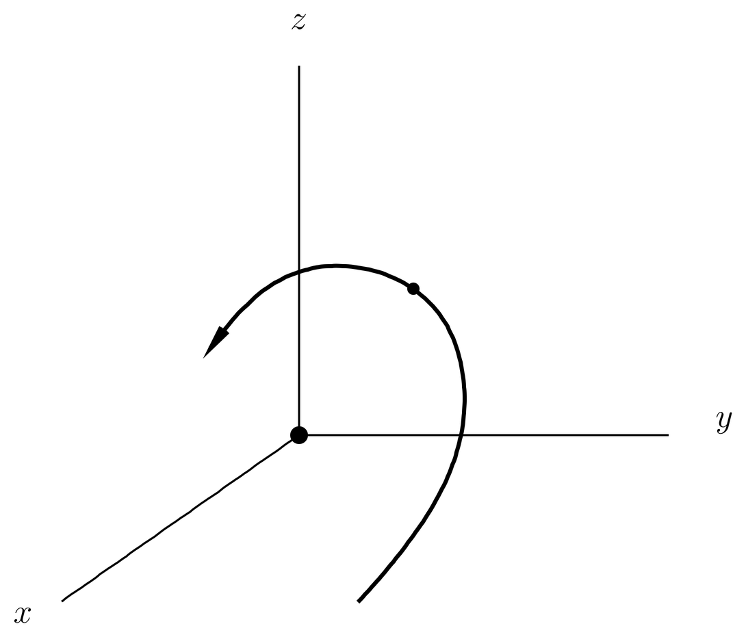
Figure 1:If the object creating a central force field is very massive, we may treat the motion of a particle in the field as a one-body problem.
The force is presumably created by some particle or physical object. We assume that its mass is infinite (or much larger than that of the particle in orbit) so that the frame attached to it is an inertial frame. Sometimes this is not a bad approximation, for example, in atoms where the nucleus is much heavier than the electrons. If this is the case, then we obtain a one-body problem for the motion of the particle, which is described by the Hamiltonian
We assume the particle is spinless, or that spin effects can be neglected. Thus the Hilbert space for the particle is the space of wave functions . In 15. Orbital Angular Momentum and Spherical Harmonics\ we developed the theory of the rotation operators and angular momentum operators that act on this space. We also found the standard angular momentum basis, which consists of radial wave functions times 's.
The Hamiltonian (1) possesses rotational symmetry, that is, it commutes with all rotation operators , whose action on wave functions is given by (13). Without going into details, this is obvious from the fact that the kinetic energy is proportional to , the dot product of two vectors, while the potential energy is a function of , where , another dot product of two vectors. Since the dot product of classical (-number) vectors is invariant under classical rotations, we expect the same for vectors of quantum operators. We will explore this question in more detail in 20. The Wigner-Eckart Theorem, but for now the basic line of reasoning should be clear. If there is any doubt, one can explicitly verify the commutators
which show that
since is a function of . Conversely, if an operator commutes with all rotations , then it commutes in particular with infinitesimal rotations, and therefore with the three components of .
As a result, commutes with the commuting operators and , so the three operators possess a simultaneous eigenbasis. From 15. Orbital Angular Momentum and Spherical Harmonics\ we already know the general form of a simultaneous eigenfunction of and ; it is
where is an arbitrary radial wave function. See (42). By demanding that this wave function also be an eigenfunction of , we can determine the radial wave function .
To do this we substitute (4) into the Schr"odinger equation for the Hamiltonian (1),
Working on the kinetic energy first and using (30), we have
But if has the form (4), then acting on the part brings out , and all terms have a common factor of . This also applies to the potential energy and total energy terms in the Schr"odinger equation, so the common factor of can be cancelled. We obtain an equation for the radial function alone,
where is the effective potential,
The effective potential is the sum of the centrifugal potential (the first term) and the true potential, . The centrifugal potential is physically the angular part of the kinetic energy, what could be written classically as
Mathematically, however, it looks like a potential and it is usually treated that way. The first term of Eq.~(7) is the radial part of the kinetic energy, what could be written classically as . (7) is called the radial Schr"odinger equation, or, as we shall call it, version one of the radial Schr"odinger equation.
Version two of the radial Schr"odinger equation is created by making the substitution
which after a little algebra results in
This version is easy to remember because it is almost the same as the one-dimensional Schr"odinger equation (usually written in terms of some variable with ). The only differences are the presence of the centrifugal potential in the radial Schr"odinger equation and the fact that lies in the range .
It is reasonable to define the normalization of the radial wave function by the integral,
because that is the radial part of the three-dimensional normalization integral
when has the form (4). Notice that this implies the normalization of the version two radial function ,
which is the usual one for the one-dimensional Schr"odinger equation apart from the range of integration.
Separation of Variables
The usual way of deriving the radial Schr"odinger equation in introductory courses is to separate the three-dimensional Schr"odinger equation in spherical coordinates. The results are the same as in The Radial Schr"odinger Equation. The method of separation of variables, when it works, is a powerful one for solving multidimensional partial differential equations that sometimes leads to exact solutions that would be difficult to find otherwise. Most wave equations are not separable in any coordinate system, however. Fortunately, many common model problems are separable in at least one coordinate system, while many others are close to a separable system and can be treated by perturbation theory. If this is not so, then usually numerical techniques will be required to find solutions. Some systems are separable in more than one coordinate system, for example, the Schr"odinger equation for all central force problems in three dimensions is separable in spherical coordinates, while the free particle is also separable in rectangular coordinates and the hydrogen atom is also separable in confocal parabolic coordinates.
In all cases, separability is related to the existence of constants of the motion, that is, operators that commute with the Hamiltonian that are related to some symmetry of the system. If the Schr"odinger equation for some multidimensional system is not separable in any coordinate system, it probably means that the system does not possess any continuous symmetries at all. It may possess discrete symmetries, such as parity and time reversal, but these do not lead to separability of the wave equation in any coordinates. If the Schr"odinger equation is separable in more than one coordinate system, it means that the system respects a larger symmetry group than that needed to ensure the solvability of the problem at all. For example, all central force problems in quantum mechanics are separable in spherical coordinates, which corresponds to the symmetry of the system under rotations. But the free particle is also invariant under translations, so the free particle Schr"odinger equation is also separable in rectangular coordinates, while the hydrogen atom, which possesses an symmetry group, is separable also in confocal parabolic coordinates.
Thus, the success of the method of separation of variables is due to some symmetry of the system, although this is usually not obvious when we apply the method. In this course we are emphasizing the symmetries and their impact on our understanding of the quantum mechanics, so we have approached the solution of several problems by studying the symmetry operators first and then studying the Hamiltonian. For example, in solving the problem of the charged particle in a uniform magnetic field, we diagonalized the operators that commute with the Hamiltonian first, whereupon the Hamiltonian was easy to diagonalize. Also, in central force motion, we diagonalized the operators and first, which led to the standard angular momentum basis, and then we turned our attention to the Hamiltonian (as in this set of notes). This approach leads to the solution of some problems or at least useful results even when the system is not separable. For example, as we shall see in Energy Eigenstates in Isolated Systems, it is possible to understand some important general features of systems with rotational invariance, including very complicated ones, with no need to talk about separating the wave equation (indeed, in some cases we do not even know what the wave equation is, only the symmetries it possesses). We will accumulate several examples of this type before the course is over. In all cases, it turns out to be a good strategy to diagonalize the symmetry operators first, and then to turn our attention to the Hamiltonian.
Quantum Numbers and Degeneracies
The radial Schr"odinger equation is parameterized by , with , because the centrifugal potential depends on . Thus we might say that there is a different radial Schr"odinger equation for each value of . The energy eigenvalues for a given value of may be either discrete or continuous. In fact, for potentials that go to 0 as , there will be a continuous spectrum above the continuum threshold at . For such potentials and for a given value of , there will always be a continuous spectrum, but there may or may not be any bound states. For example, in the case of the deuteron, which is approximately a central force problem involving a proton and a neutron, there is one bound state for , and none at all for any higher values of . (However, spin-dependent forces are important in the case of the deuteron, and the system is not purely a central force problem.)
Assuming there are bound states, let us denote their discrete eigenvalues by , where just sequences the levels for a given value of , using some scheme. Thus, the energy depends on two quantum numbers, and , but not on . Similarly, the radial wave functions or depend on the same two quantum numbers, so we shall write or to emphasize this. The total wave function is
The radial Schr"odinger equation shares some features with the usual one-dimensional Schr"odinger equation, for example, if vanishes anywhere on the interval then the eigenfunctions are nondegenerate. See Degeneracies in One Dimension. But for realistic potentials goes as as (see Behavior of the Radial Eigenfunctions Near ), so and the radial eigenfunctions are nondegenerate, in both the bound and unbound cases. Of course the bound eigenfunctions also go to zero as . We see that the discrete eigenvalues are distinct, that is, nondegenerate, for a given value of . The nondegeneracy we are referring to here concerns the eigenvalues and eigenfunctions of the radial Schr"odinger equation for a given value of , regarded as a one-dimensional wave equation.
When we consider the three-dimensional Schr"odinger equation, however, and include the angular quantum numbers, then degeneracies appear. That is, the energies are at least -fold degenerate because they do not depend on . Physically this is due to the fact that the energy of the system does not depend on the orientation. The quantum number indicates the projection of the angular momentum onto the -axis. But if we rotate our system (or the axes), this projection changes. Therefore the energy eigenvalues cannot depend on .
There could be further degeneracies, however. It is possible that some could be equal for different values of , in which case the degeneracy would be higher than . For a randomly chosen potential , this is not very likely, since the different radial wave equations for different values of have spectra that are effectively independent of each other. Generically, the degeneracies are just for each , no more than what is predicted by rotational invariance alone.
For some potentials, however, there are systematic degeneracies among different for different values of and . This applies to the Coulomb potential and the harmonic oscillator potential . The harmonic oscillator we are referring to is the three-dimensional, isotropic harmonic oscillator. There are no other examples in three-dimensional central force motion. In both cases, the extra degeneracy is due to some extra symmetry that goes beyond ordinary (rotational) invariance. For the Coulomb potential, the symmetry group is , while for the three-dimensional, isotropic harmonic oscillator, it is . In the case of hydrogen, the extra degeneracy applies only in the electrostatic, spinless, nonrelativistic model, in which the energy levels are proportional to , where is the principal quantum numbers. The extra degeneracy appears in the fact that these levels are independent of . As we add extra physical effects, coming closer to a realistic description of hydrogen, we will see the extra degeneracy gradually disappear. When all physical effects are included, hydrogen, too, has only the -fold degeneracy expected on the basis of rotational invariance.
Behavior of the Radial Eigenfunctions Near 
The behavior of the radial wave function for small is often important in applications. Let us assume the potential is either well behaved at the origin or that if it diverges it does so no faster than . This covers the important case of the Coulomb potential. Let us also assume that the wave function goes as for some power near , something we will write as . This means that for some constant plus other terms that go to zero more rapidly than as , or, equivalently,
Then for small we have
and
As for the term , it behaves at worst as as , so it is negligible compared to the terms (17) and (18) as . The same is true for the term , which behaves as as . The dominant terms in the radial Schr"odinger equation at small come from the kinetic energy alone (including the centrifugal potential). Since these terms have to cancel, we have
This has two solutions,
The solution is not acceptable when , because then would have a nonintegrable singularity at , that is, the wave function would not be normalizable and there would be an infinite amount of probability in a small neighborhood of . As for the case , this would result in near , which would not satisfy the Schr"odinger equation at because
That is, the kinetic energy in the 3-dimensional Schr"odinger equation would contain a -function, and for the Schr"odinger equation to be satisfied, that -function would have to be cancelled by another -function in the potential energy.
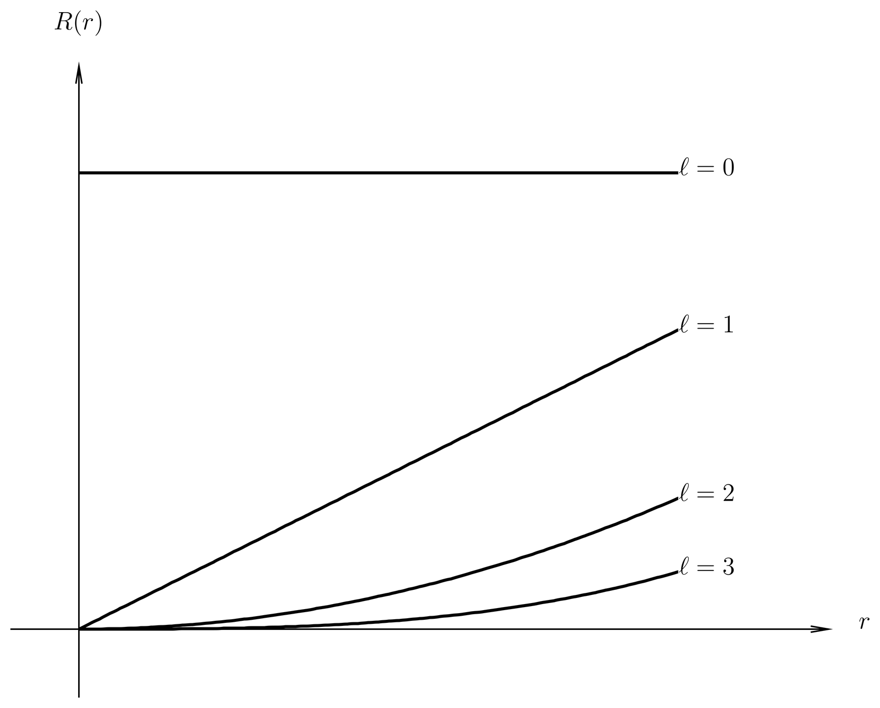
Figure 2:The radial wave function behaves as near . It lies down ever more flat against the -axis as increases. This is only the leading behavior of for small ; as increases, correction terms become important.
Thus, the only possible solution of (19) is , and we see that the radial wave function has the behavior
near . The leading behavior depends only on the angular momentum quantum number . This is a simple rule that is often important in practice. It means that the radial wave function lies down more and more flat near as increases (see Figure 2), and that the probability of finding the particle in some small neighborhood of goes to zero exponentially as increases. This applies, for example, to the probability of finding an atomic electron inside the nucleus.
Free Particle
Let us now take the case of the free particle, . In this case there is no question of the mass of the object that creates the force field, since there is no force. The free particle Hamiltonian is symmetric under both translations and rotations, so a complete set of commuting observables can be chosen in more than one way. If we choose as the complete set, then the simultaneous eigenstate is
a plane wave with . The energy is given in terms of the momentum eigenvalues by
The spectrum is continuous with .
If we choose as the complete set, then we must solve the radial Schr"odinger equation with . This is easier in version one, (7). Expressing the energy in terms of a wave number by
and writing for a dimensionless radial variable, the radial Schr"odinger equation becomes
This is the standard differential equation for the spherical Bessel functions. These come in two types, denoted and (see Abramowitz and Stegun, Chapter~10).
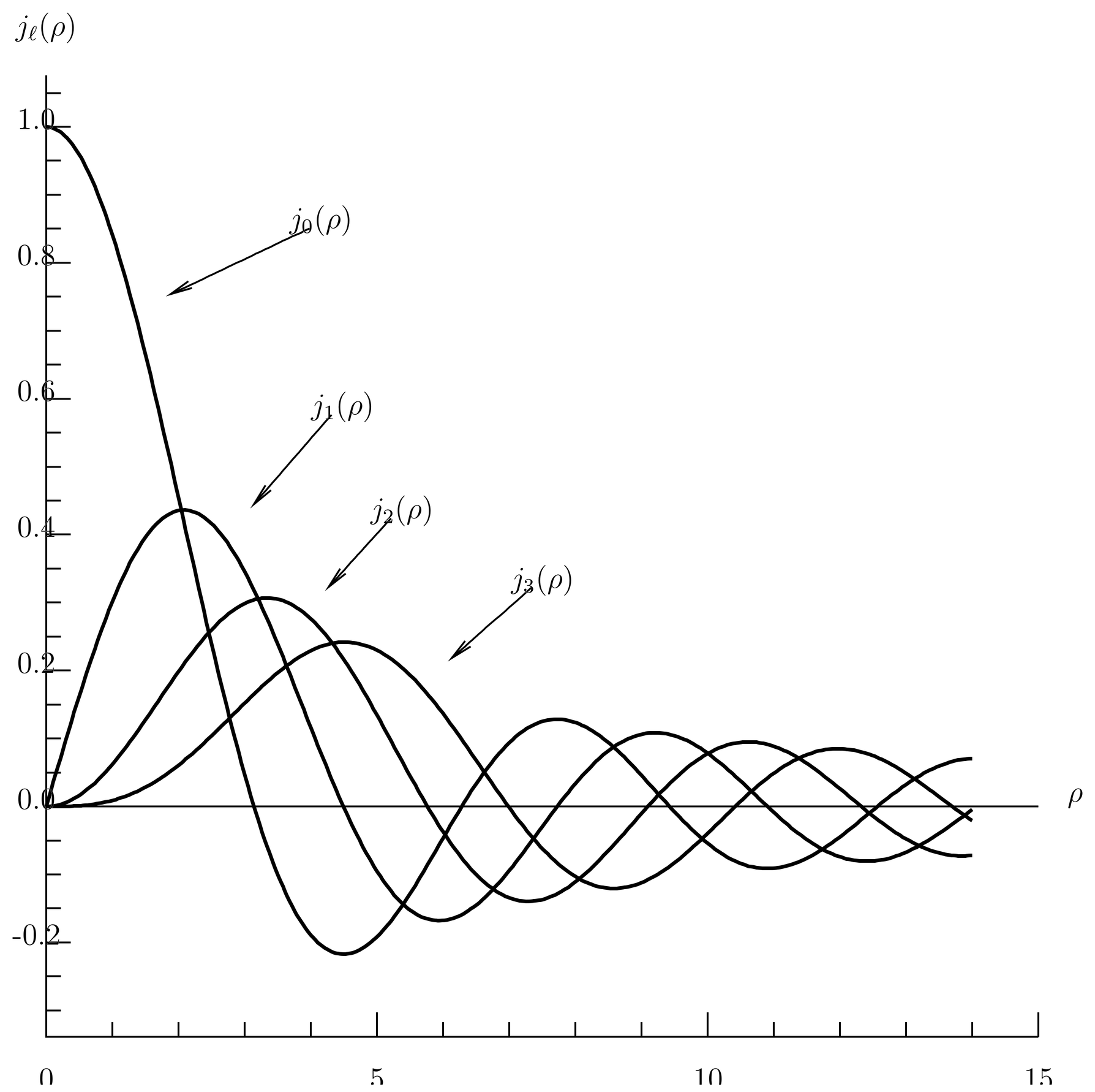
Figure 3:Spherical Bessel functions for different values of .
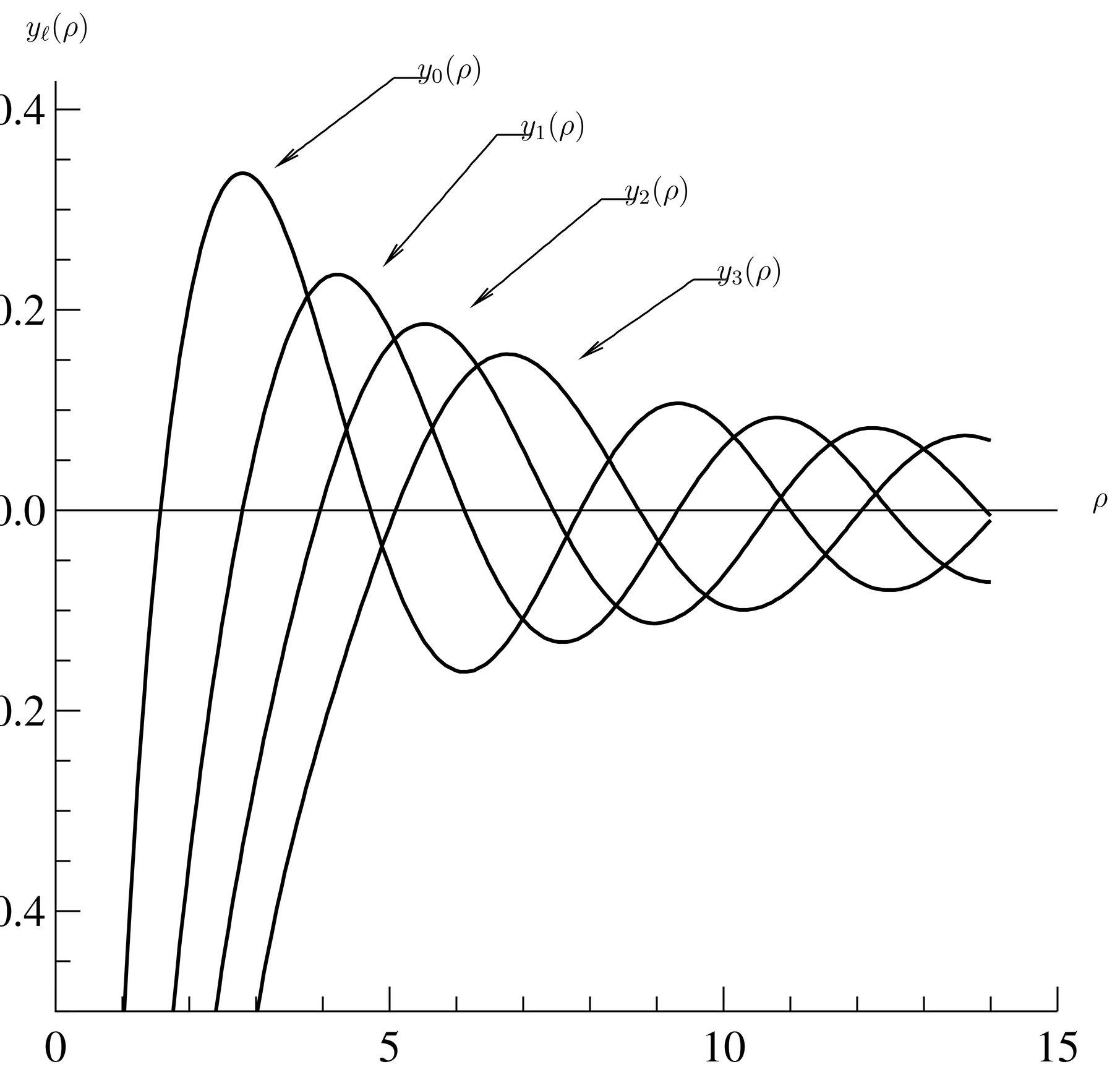
Figure 4:Spherical Bessel functions for different values of .
The functions are regular at the origin and so are physically acceptable solutions for the free particle. Some examples are plotted in Figure 3, which clearly shows the behavior near . The functions diverge at the origin and so are not acceptable free particle solutions if the particle is able to reach the origin. They are plotted in Figure 4. On the other hand, the -type spherical Bessel functions are useful in scattering theory where at large distances from the origin the particle becomes free, and it is desired to represent an arbitrary solution of the Schr"odinger equation in that region. Since there is no attempt to extend those solutions all the way down to , the -type solutions are acceptable (and necessary) in that case.
Limiting Forms of the Spherical Bessel Functions
Many problems involving special functions can be solved knowing only the limiting forms for large and small values of the arguments. In the case of the spherical Bessel functions, the limiting forms at small are
See Abramowitz and Stegun, Eqs.~(10.1.2) and (10.1.3). As for , we see the small rule (22), to within a constant (which we couldn’t have guessed anyway because it is conventional). As for , we see the solution of (19) that we rejected earlier as nonphysical.
The limiting forms at large (actually, ) are
See Abramowitz and Stegun, Eqs.~(10.1.1), (9.2.1) and (9.2.2). These are useful in scattering theory.
WKB Theory and Spherical Bessel Functions
The limiting forms at large can be obtained by treating the radial Schr"odinger equation (in version two) by one-dimensional WKB theory, apart from normalization. We discuss this briefly without going into details because WKB theory provides an easy way to understand all the qualitative features of the functions and , as seen in Figs.~Figure 3 and Figure 4.
It turns out that the accuracy of the WKB approximation for radial wave equations is improved if the quantity is replaced by . This is called the Langer modification, and it has to do with the singularity in the centrifugal potential at . That is, for the purposes of WKB theory, we work with the effective radial potential,
The centrifugal potential cannot be turned off and is present even for a free particle (except when ). Thus the effective potential depends on , and we have different turning points etc depending on . In the case of the free particle () the turning point is the solution of
or,
The turning point moves out as increases, something that can also be seen from Figure 5.
It might seem strange that a free particle should have a turning point at all. The only reason it does is the centrifugal potential, which, as mentioned, is really a part of the kinetic energy. Figure 6, which shows a classical orbit of a free particle of some energy and angular momentum , helps explain the situation. The orbit is a straight line which must pass at some minimum distance from the origin. In the figure, the orbit lies in the - plane. The minimum distance is . The family of all possible classical orbits of the given and is a set of straight lines tangent to the sphere . In quantum mechanics, the minimum radius becomes the radial turning point .
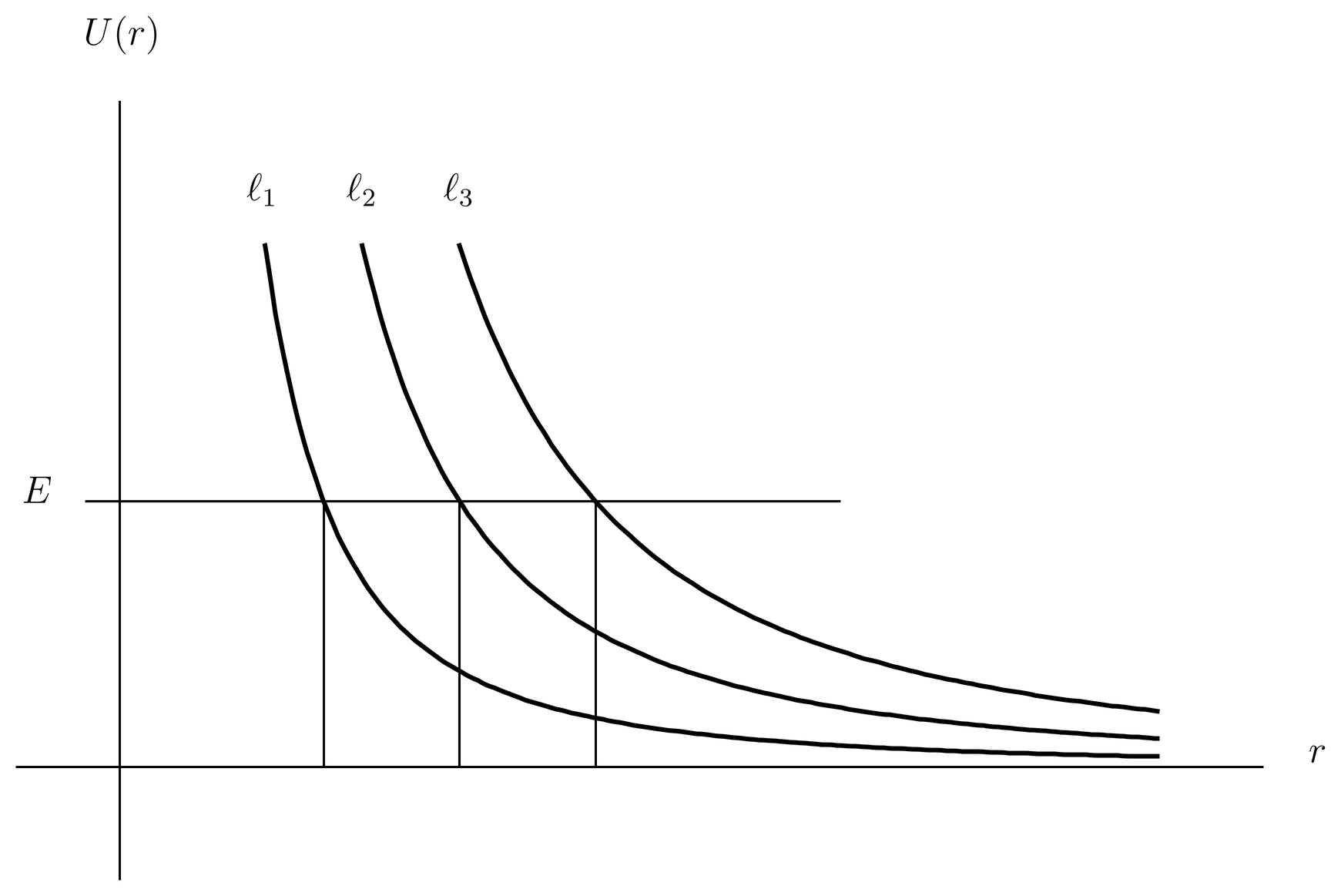
Figure 5:The radial turning point for a free particle moves out as increases.
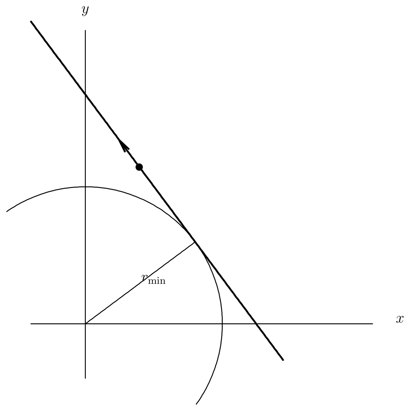
Figure 6:The minimum distance of approach to the origin of a classical free particle of momentum and angular momentum is .
For the exact spherical Bessel functions , which are 0 at , rise up to a first maximum somewhat after the point , and then oscillate beyond that. From the standpoint of WKB theory, we have a classically forbidden region to the left of the turning point , an Airy-function type of behavior in the neighborhood of the turning point (see Fig.~\figr\wkb.8), and a classically allowed region to the right, exactly as we would expect on the basis of Figure 5. The case is an exception, since in that case the centrifugal potential vanishes and there is no turning point.
The functions can also be understood from the standpoint of WKB theory; these are the functions that diverge exponentially as we move into the classically forbidden region (that is, as we move to the left of the turning point at ), and have the behavior of the function in the neighborhood of the turning point (see Fig.~\figr\wkb.9).
It will be left as an exercise to work out the details of the WKB approximations to the spherical Bessel functions. The WKB solutions turn out to be more accurate than (29) and (30) when is not too much larger than , but go over to them in the limit .
Two-Body Central Force Motion
We return to the discussion of The Radial Schr"odinger Equation. If the source of the force field is not infinitely massive, then a coordinate system attached to it is not an inertial frame and we must take into account the dynamics of the force center itself. That is, we must deal with a two-body problem, which we describe in an arbitrary (“lab”) inertial frame. We let and be the coordinates of the two particles with respect to this frame, with masses and , respectively. We assume the force is described by a potential
which depends only on the distance between the particles. The Hamiltonian is the sum of the kinetic and potential energies,
where and are the momenta of the two particles.
We assume the particles are spinless or else we ignore spin. We write for the configuration space wave function, upon which the operators act as differential operators,
Translation operators act on the wave function according to
a two-particle, three dimensional generalization of (24). The generator of translations is the total momentum,
The Hamiltonian commutes with all translations because the distance between the particles is not changed when both particles are displaced by the same amount. Therefore also commutes with the total momentum,
The Hamiltonian is also invariant under rotations. Rotation operators act upon according to
as explained in \orbamsph.9. The angular momentum of the system (the generator of rotations) is
where
that is, it is the sum of the angular momenta of the two particles. The Hamiltonian (35) commutes with all rotations and hence with the total angular momentum ,
To solve the Schr"odinger equation for Hamiltonian (35) we introduce a change of coordinates,
where
is the total mass of the system, so that is the position of the center of mass and is the relative position vector between the particles. We write for the wave function transformed to the new coordinates. We also define momenta “conjugate” to and as the differential operators,
when acting on wave functions . By the chain rule, we can express the momenta and of the particles in the lab frame in terms of and ,
or,
Solving these for and , we find
and we see that defined by (47) is the total linear momentum of the system (the generator of translations), as in (38). The transformation specified by (44), (45), (52) and (53) is an example of a “canonical transformation,” that is, one which preserves the canonical commutation relations. That is, we have
where and refer to the components of and , respectively. We see that any function of commutes with any function of .
Transforming the Hamiltonian (35) to the new coordinates is straightforward. As for the potential, it becomes , where is the distance between the two particles. Also transforming the kinetic energy, we find the Hamiltonian as a sum of a center-of-mass term and a relative term,
where
and
Here is the reduced mass, defined by
The reduced mass is the harmonic mean of the masses and . If one of the two particles is much more massive than the other (for example, in hydrogen where the proton is roughly 2000 times more massive than the electron), then the reduced mass is closer to the mass of the lighter of the two particles (for example, the electron, in the case of hydrogen). At the other extreme, if the two masses are equal, , then .
The Hamiltonian is a free particle Hamiltonian, containing physically the kinetic energy of the center of mass, while is physically the kinetic energy about the center of mass plus the potential energy. The two Hamiltonians and commute with each other,
because they are functions of different degrees of freedom, and they also commute with the total Hamiltonian . Thus, and possess a simultaneous eigenbasis, which is also an eigenbasis of the total Hamiltonian .
This simultaneous eigenbasis consists of functions of the form,
a product of a center-of-mass wave function times a relative wave function . Each of these are eigenfunctions of their respective Hamiltonians,
where the eigenvalue of the total Hamiltonian is given by
The center-of-mass equation (61) is easy to solve since is just a free particle Hamiltonian. For example, if we choose the three components of as a complete set of commuting observables for the center-of-mass motion, we have eigenfunctions
that is, plane wave with momentum (being somewhat sloppy about the distinction between the operator and its eigenvalues). Of course we may also solve this free particle equation in spherical coordinates.
The relative wave equation (62) has the form of a pseudo-one-body problem of the kind considered earlier in these notes, but with a reinterpretation of the variables. Now is the relative position vector between the two particles, and is defined by (53). Also, the mass used earlier in these notes must be identified with the reduced mass . In the limit while holding fixed, we recover the earlier results in which we had an infinitely massive force center. It is worthwhile keeping in mind, however, that in real problems the position and momentum operators for relative motion in a two-body problem such as hydrogen are really functions of the positions and momenta of both particles.
As a final remark, we transform the total angular momentum of the system , expressed in terms of the coordinates of the two particles in (41) and (42), over to the new coordinates. We find
where
The Hamiltonian commutes with , and commutes with . In other language, the total Hamiltonian commutes not only with overall rotations of the system, but with rotations of the center of mass and with rotations about the center of mass separately.
The Rigid Rotor
As an example of central force motion we consider the rigid rotor. We have already considered the rigid rotor in a plane (see Other Types of Turning Points), but now we consider it in three dimensions. The rotor consists of two masses and connected by a massless, rigid rod of length , as in Figure 7. This is an example of central force motion because the constraint can be thought of as due to a sharply confining potential centered on .
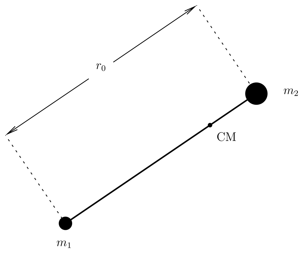
Figure 7:A rigid rotor in which the two masses and are separated by a fixed distance . The center of mass is closer to the more massive end.
First we look at the classical mechanics. The moment of inertia about the center of mass is
The energy is
It is the same as the centrifugal potential, which is logical since the centrifugal potential is really the angular part of the kinetic energy, which is all there is for a rigid rotor.
The classical configuration, apart from the center-of-mass degrees of freedom, is just the orientation of the rotor, specified by angles . This suggests that the wave function in quantum mechanics should be (with no -dependence). As for the quantum Hamiltonian, we guess that it should be
the obvious operator corresponding to the classical energy (68).
This makes it easy to solve the Schr"odinger equation, . The energy eigenvalues are
and the eigenfunctions are
The energies do not depend on the magnetic quantum number , and are -fold degenerate.
Diatomic Molecules
Rigid rotors are an idealization that does not exist in nature, but diatomic molecules exist and have many similar features. Consider, for example, carbon monoxide (CO). The atomic masses are , , where is the mass of the hydrogen atom, with , where is the mass of the electron. We denote the reduced mass of the carbon-oxygen system by (rather than as above, since we wish to contrast the large mass with the small electron mass ). Numerically,
very roughly. This leads to some small parameters that we will see in the analysis of the molecule,
where very rough values are given. These values apply very roughly to most common diatomic molecules.
A diatomic molecule can be regarded as a central force problem involving two bodies (the atoms), each treated as a particle. Of course the particles in question are composite, made up of nuclei and electrons, but in a certain approximation they may be treated as independent units, that is, particles in their own right. The more elaborate theory that justifies this is called the Born-Oppenheimer approximation.
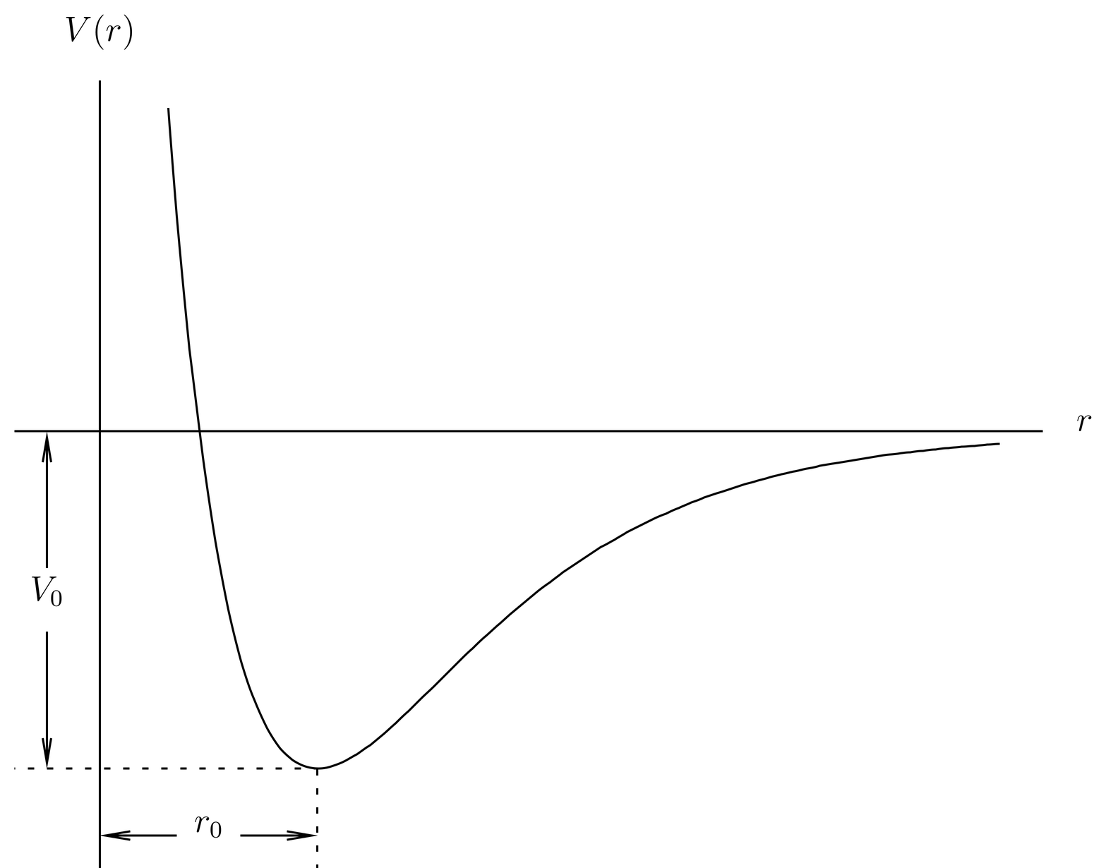
Figure 8:Typical potential in a diatomic molecule. The equilibrium radius is , the well depth is .
The potential of interaction of two atoms in a diatomic molecule is sketched in Figure 8. The potential is strongly repulsive at short distances, because as the two atoms are brought together their electron clouds overlap and by the Pauli principle the electrons are forced into higher energy states. It is the same principle at work as when a degenerate electron gas is compressed; the short range repulsion of two atoms can be thought of as due to the pressure of a degenerate electron gas. At large distances the force is mostly electrostatic, and is attractive. Each atom causes the other atom to polarize, creating an attractive dipole-dipole interaction. In between these two effects compete with one another, creating a potential well. The potential is characterized by two parameters, the well depth and the equilibrium radius (that is, is the distance to the minimum of the potential, which classically would be an equilibrium radius). For CO the actual values are , .
There is no simple analytical form for , so we will rely on order-of-magnitude estimates that follow from dimensional analysis. The basic fact we rely on is that the force between the atoms is determined by the dynamics of the electron clouds. There are only three fundamental constants that enter into the electron dynamics: , and . The speed of light is not on the list because the interaction is electrostatic and the electron motion is nonrelativistic. It is important to note that the nuclear masses do not enter into the potential. One might wonder whether some dimensionless parameters are important, such as the number of electrons in the atom, or, equivalently, the nuclear charges (6 for C and 8 for O). The answer is that these numbers are not as important as one might expect, because the atomic interactions, at the distances we are interested in, are mediated mostly by the valence electrons. Inside the typical radius of the valence electrons is the atomic core, consisting of electrons that shield and nearly neutralize the positive charge from the nucleus.
From , and it is possible to construct a unique distance, energy, time, etc. These are displayed in Table 1. These are the same values of distance, energy, etc, that appear in the hydrogen atom, and for the same reason: the only physical constants we have to work with are , and . For example, is the Bohr radius and is twice the ionization potential of hydrogen (). Notice in particular : it is the velocity of the electron in the ground state of hydrogen. Although fast, it is still nonrelativisitic (). As claimed, the electrons are nonrelativistic.
Table 1:Characteristic distance, time, etc for electron dynamics in an atom.
Dimension | Definition | Value |
|---|---|---|
distance | ||
energy | ||
velocity | ||
frequency | ||
time |
Returning to the CO potential in Figure 8, the well depth should be of the same order of magnitude as ; in fact, it is about 40%. Also, should be of the same order of magnitude as ; in fact, it is a little more than twice as big. For an order-of-magnitude estimate, the agreement is not bad.
The radial Schr"odinger equation in our potential is
At first we take , so we have a one-dimensional Schr"odinger equation with potential . Since there is a well we expect bound states, which physically are the quantized vibrations of the molecule. We can approximate the potential near the bottom of the well by a harmonic oscillator potential, that is, we can write
where is the frequency of small vibrations. Figure 8 shows that as the energy is raised much above the bottom of the well the parabolic approximation ceases to be a good one, but if there are many bound states then we can expect the low-lying ones to be described at least roughly by the harmonic approximation. In a moment we will estimate the number of bound states.
We can estimate the parameter in (75) by supposing that when , then the potential is near dissociation, that is, is near zero. Dropping factors of etc, this gives
or,
where is given by Table 1. As long as the harmonic approximation is valid, the vibrational energy levels are , where is the vibrational quantum number.
The vibrational frequency of the molecule is down by a factor of the square root of the mass ratio, roughly 10-2 according to (73), in comparison to the typical frequency of the electronic motion . Frequency is also (as an order of magnitude) the frequency of a photon emitted or absorbed in a transition between electronic states, while the energy difference between two neighboring levels of the vibrational harmonic oscillator is , that is, the emitted or absorbed photon has frequency . Thus, vibrational transitions involve photons of energy roughly 100 times smaller than electronic transitions. Electronic transitions are typically in the visible to ultraviolet range of frequencies, while vibrational transitions are in the near to mid infrared.
We can estimate the number of bound vibrational states by taking the ratio,
This is roughly the value for many diatomic molecules.
In the vibrational ground state the wave function is a Gaussian of width (where “ho” means “harmonic oscillator”), which according to (12) is given by
In the ground state the wave function occupies roughly 10% of the bond length. The molecule does behave like a rigid rotor at least approximately, because the interatomic separation lies in a narrow range near .
To account for the case , we must include the centrifugal potential. But since the wave function occupies only a small part of the -axis near , the centrifugal potential is nearly constant over the extent of the wave function and we can just replace by in the centrifugal potential:
where is the moment of inertia in the equilibrium position. We see the appearance of the energies of the rigid rotor, derived in an intuitive way in The Rigid Rotor. The replacement (80) will become less accurate as increases (because the vibrational wave function is more spread out), or as increases (because the centrifugal potential becomes more rapidly varying in ).
With the replacements (75) and (80), the radial Schr"odinger equation becomes
This is a harmonic oscillator with shifted origin and a constant term ( plus the centrifugal potential) added. The energy eigenvalues are immediate:
This is only valid for small and , but it does give an easy and roughly accurate picture of the rotational and vibrational spectrum of the molecule. Notice that the energies have the general form predicted for central force potential in Quantum Numbers and Degeneracies, that is, they depend on both and .
Let’s examine the spacing between rotational energy levels in order to estimate the energy of the photon emitted or absorbed in a rotational transition. We define as the spacing between the and levels, or,
This is roughly 100 times smaller than , and roughly 10,000 times smaller than the energy of an electronic transition. The photons emitted or absorbed in rotational transitions typically lie in the far infrared to microwave range.
The molecule has three different energy scales: that of , involved in electronic transitions, or equivalently, the energy of dissociation of the molecule (breaking the bond); the vibrational energy , roughly the square root of the mass ratio times smaller; and the energy of rotational transitions, roughly the square root of the mass ratio times smaller still.
Greenhouse gases absorb infrared radiation from the earth by making vibrational transitions in molecules. These are not usually diatomic molecules, because the stretching vibrations of molecular bonds typically have too high a frequency. In addition, the main molecular species in the atmosphere, and , are homonuclear diatomics without a permanent electric dipole moment. Instead, the greenhouse culprits are mainly and , triatomics that have bending and twisting modes of lower frequency.
Problems
Problem 1.
Consider central force motion in two dimensions. The wave function is , where are plane polar coordinates specified by
(a) Find the most general function that is an eigenfunction of . Express it in terms of a radial wave function , along the lines of what is done in the notes for the three-dimensional case. What is the spectrum of ?
(b) Consider a central force Hamiltonian in two dimensions,
where . In this problem is the mass of the particle, while is the quantum number of . Show that this Hamiltonian commutes with . Therefore simultaneous eigenfunctions of and exist.
By expressing the Laplacian in polar coordinates and using the result of part~(a), find a radial wave equation for that will determine energy eigenfunctions and eigenvalues.
(c) Define a modified radial wave function by
where is a power to be determined. Determine by requiring that the modified radial wave equation should look like the one-dimensional Schr"odinger equation, apart from the range of the variable and the presence of the centrifugal potential.
(d) Consider the case of the free particle. Express the radial eigenfunctions in terms of ordinary Bessel functions, , and in terms of the energy and the quantum number of . You will have to look up the differential equation for ordinary Bessel functions.
(e) For any potential that is not too badly behaved near the origin, find the dependence of the radial eigenfunction near . Verify that the free particle solutions of part~(d) satisfy this condition.
Problem 2.
A good physicist has a feel for orders of magnitude of various physical quantities. Let’s look at some real numbers for the carbon monoxide molecule (CO). We’ll see if it is effective as a greenhouse gas, scattering infrared photons either by making vibrational or rotational transitions.
(a) The potential well is illustrated in Figure 8, with , . Approximate the potential near the bottom of the well by (75), with some vibrational frequency . By assuming that (dissociation) when , solve (75) numerically for . Compare to the experimental value, which is . Note that . How well does the order-of-magnitude estimate (77) work? See Table 1 for .
(b) What is the probability that the CO molecule is in the vibrational state at 300 Kelvins? A typical infrared photon trying to escape the earth’s atmosphere has an energy of 300K. There is not much CO in the atmosphere (good thing, since it’s poisonous), but if there were, would it be efficient at absorbing or scattering photons by making vibrational transitions? Such absorption or scattering would impede the escape of heat from the earth, creating a greenhouse effect.
(c) A CO molecules makes a transition from the to the rotational state. What is the frequency (in Hertz) of the photon emitted? Compare to the vibrational frequency in part (a), and note the rough estimates made in Diatomic Molecules. What is the most probable value of in CO gas at 300K? Absorption or scattering of photons by rotational transitions is most probable when , and falls off rapidly for higher values of . Is CO at 300K effective at scattering typical infrared photons at 300K, by making rotational transitions?
Problem 3.
Consider the helium atom in a lab frame. The positions of the nucleus, electron 1 and electron 2 are , and respectively. The mass of the nucleus is and that of the electron is . Thus the laboratory Hamiltonian is
We will only be interested in the kinetic energy in this problem.
Let } be the center of mass position and let
so that and are the positions of the two electrons relative to the nucleus. Also define new momentum operators,
Express the kinetic energy as a function of these new momentum operators. You will obtain a term proportional to . This is called a “mass polarization” term.
The usual simple-minded treatment of helium treats the nucleus as infinitely heavy. In this approach there are no mass polarization terms. Explain why its a good approximation to neglect those terms (thus, the usual approach is ok).