04. Spatial Degrees of Freedom
Introduction
In these notes we develop the theory of wave functions in configuration space, building it up from the ket formalism and the postulates of quantum mechanics. We consider a system with one particle moving in space. In this set of notes we will not deal with the dynamics of the particle, so we will not need to say what the Hamiltonian is (that is taken care of in 05. Time Evolution in Quantum Mechanics). We assume the particle has no spin or other internal degrees of freedom, or that if such degrees of freedom exist they can be ignored. This allows us to establish an isomorphism between the Hilbert space of kets and the Hilbert space of wave functions on configuration space. We then introduce translation operators and use them and the classical correspondence to motivate the definition of momentum in quantum mechanics. We then explore the two representations, position and momentum, and the relationship between them. Finally, we discuss minimum uncertainty wave packets.
The Position Representation; Wave Functions
For simplicity we begin with the one-dimensional case, in which the physical system is a particle moving in one dimension. According to the postulates of quantum mechanics, this system is associated with a Hilbert space . We assume the position of a particle in one dimension can be measured, and that the results of the measurement are continuous. Thus, we are dealing with the case of the continuous spectrum. We denote the operator corresponding to measuring by , so the eigenvalue-eigenket problem is
Here is the operator, is the eigenvalue, and is the eigenket with eigenvalue . Since belongs to the continuous spectrum, the eigenkets are not normalizable and lie outside Hilbert space.
We also assume that by itself forms a complete set of commuting observables, which, as we shall see, means that the wave function is a scalar (it has only one component). In practice, this means that we are dealing with a spinless particle (a particle of spin 0, for example, the -meson, the nucleus of ordinary helium, or the hydrogen atom in its ground state). It may also mean that we have a particle with spin, such as the electron, but the spin degrees of freedom are not important for the physics we are interested in. This point was discussed in Resolving Degeneracies; Complete Sets of Commuting Observables.
Since is a complete set of commuting observables, the eigenkets are nondegenerate and form a basis in the Hilbert space in the continuum sense. These eigenkets are only defined by (1) to within a normalization and a phase. We fix the normalization by requiring
the usual orthonormality condition in the continuum. The phase conventions for the eigenkets are a question we shall return to later. Under these assumptions, the resolution of the identity takes the form
Now let represent a normalized (pure) state of the system, let be an interval on the -axis, and let be the corresponding projection operator,
Then, according to the postulates of quantum mechanics (Postulates of Quantum Mechanics (Incomplete Form)), we have
We now introduce the definition,
of the wave function , whereupon the probability (5) can be written,
Since the interval is arbitrary, we see that must be interpreted as the probability density of finding the particle on the -axis. We have derived wave functions from the ket formalism plus the postulates of quantum mechanics, as promised in 01. The Mathematical Formalism of Quantum Mechanics.
(6) is important because it shows how to go from kets to wave functions. It takes the place of sloppy notation such as (7). That is, in addition to the Hilbert space of kets, we have another Hilbert space, this one consisting of normalizable wave functions on configuration space, . (6) expresses the mapping between these spaces, which identifies kets with wave functions. To go the other direction, we multiply on the left by the resolution of the identity (3),
which, by using (6), becomes
This is the inverse of (6), allowing one to go from a wave function to the corresponding ket . We see that is the set of expansion coefficients of the ket in the position eigenbasis.
Another consequence of this formalism follows easily. Suppose we have two kets and , and we wish to compute the scalar product in wave function language. We simply insert the resolution of the identity (3) between the bra and the ket to obtain,
a familiar formula that translates the scalar product on the Hilbert space of kets into the language of wave functions.
This formalism is easily generalized to three dimensions. Let be a position vector in three-dimensional space, with components or . The measurement of the three components of position corresponds to a vector of operators, which we denote by (with a hat), to distinguish the operators from their eigenvalues (the results of the position measurement). In quantum mechanics, when we speak of a “vector operator” we usually mean a vector of operators, in this case three operators . We assume that the components of commute with one another,
which as explained in 02. The Postulates of Quantum Mechanics\ can be tested experimentally. For example, if we filter a beam in and then by means of small slits, or do it in the reverse order, we find that the statistical results of arbitrary measurements on the filtered beam are the same in both cases.
As above we assume that we can ignore any internal degrees of freedom of the particle, so that the three operators by themselves form a complete set of commuting observables. Then the simultaneous eigenkets of are nondegenerate and form a basis by themselves. The eigenket-eigenvalue problem is
for , a set of three simultaneous equations satisfied by an single eigenket , labeled by the three eigenvalues of the three commuting operators. In obvious generalizations of the one-dimensional case, we normalize these kets according to
we have a resolution of the identity,
and the transformation between wave functions and kets is given by
and
Also, the probability that the particle will be found in a region of three-dimensional space is
so must be interpreted as the probability density.
Equations (6) or (15) define the wave function or , respectively, in quantum mechanics. A question that arises sometimes when solving the Schr"odinger equation is whether is single-valued. But by our definitions, or is automatically single-valued, since it is just the expansion coefficient of the state with respect to the basis or .
Equations~(6) and (9) (in one dimension) or (15) and (16) (in three dimensions) make explicit the transformations back and forth between the Hilbert space of ket vectors and the Hilbert space of wave functions or . As discussed in Dirac Ket Notation, we regard these two Hilbert spaces as isomorphic but distinct, and we say that the space of wave functions or forms the configuration representation of the space of kets . There are other representations, and while the configuration representation is often used in practice one should note that in the postulates of quantum mechanics there is no privileged role assigned to it. Any calculation that can be carried out in the configuration representation can be carried out in any other representation with the same results from a physical standpoint.
In effect, a representation is merely a choice of basis, allowing one to work with the expansion coefficients of a state vector with respect to the chosen basis instead of the abstract ket vectors themselves. As noted below (9), the configuration space wave function or is the expansion coefficients of the state ket with respect to the basis of position eigenkets or . In quantum mechanics we frequently choose as a basis the simultaneous eigenkets of a complete set of commuting observables; thus, the basis is labeled by the observables in question, and we speak, for example, of the position representation, momentum representation, etc. Nothing prevents us from using other bases, however (which have no correspondence with any simple set of commuting observables).
Just as the wave function represents the ket vector in the configuration representation, so also is there a representation of various operators that act on ket vectors. Consider, for example, the operator (working in one dimension for simplicity). We know that the ket corresponds to the wave function . What wave function does the ket correspond to? Let , so that
where we have used , the Hermitian conjugate of (1). We see that the effect of multiplying a ket vector by the operator is to multiply the corresponding configuration wave function by . That is, we can write
As we say, the operator is represented by multiplication by in the configuration representation. It is represented by other operations in other representations. Similarly, in three dimensions we have
You may worry about the physical meaning of the unnormalizable eigenkets or . In reality we never measure the position of a particle exactly, instead the best we can do is to localize it in some small region of space. The eigenkets or are an idealization of this process, in which the size of the region is allowed to approach zero. This limit also leads to singular mathematics, since the eigenkets or have infinite norm and do not belong to Hilbert space.
Measuring the position of a particle is really a nonrelativistic concept, because as we localize a particle to smaller and smaller regions, by the uncertainty principle the momentum increases, ultimately taking on relativistic values. Then processes such as the creation of particle-antiparticle pairs come into play, and we are really dealing with a multi-particle situation, which is properly handled by the methods of quantum field theory. We will find later in the course that the position operator for a particle in relativistic quantum mechanics is one that is fraught with difficulties. The position operator is really a nonrelativistic concept.
Translation Operators
The subject of position measurements leads naturally into the question of translational invariance. The energy and other physical properties of an isolated system do not change if it is moved somewhere else, a fact that is more precisely stated by saying that the Lagrangian or Hamiltonian of such systems is invariant under spatial translations. This symmetry in turn leads to the conservation of momentum, which first appeared in physics as Newton’s third law.
If a system is not isolated then its energy does depend on its position, for example, the potential energy of an electron in an electric field changes if the electron is moved. But the electric field is created by other charges somewhere else, and if those charges are included in the “system,” then the energy does not change when the entire system is moved.
In summary, spatial translations are a fundamental symmetry of nature which is closely related to the law of conservation of momentum. We now develop translation operators in quantum mechanics, working initially in one dimension for simplicity.
Let be a displacement. We imagine a displacement operation as one that acts on a physical system, moving all particles from their initial positions (say, ) to their new positions (), both measured relative to an inertial frame. This is sometimes called the active point of view, because our operations take a given physical system and transform it into a new system, in this case in a different location.
In quantum mechanics, we can define a translation operator which carries out this operation on a physical system. The translation operator is a linear operator acting on the Hilbert space of a physical system, parameterized by the displacement . We define the translation operator in one dimension by
This definition makes sense, because physically is the state of the system after a measurement has placed the particle in a small region around position , and similarly for . (21) is actually a definition of the operators because the kets form a basis. If we specify the action of a linear operator on a set of basis vectors, then by linear superposition its action on an arbitrary vector becomes known.
(21) gives the action of the translation operator on the position eigenkets. Let us also work out its action on wave functions. Let be a state with wave function , and let be the translated state with wave function . What is the relationship between the old wave function and the new one ? We answer this by writing
where we have inserted a resolution of the identity, used (21) and (2), and carried out the integral. We write the result as
where we have replaced by . This is a companion to (21), which gives the action of translation operators on the basis kets; this gives their action on wave functions.
There are several remarks concerning (24). First, notice the minus sign in this equation, compared to the plus sign in (21). The minus sign is necessary to get a wave function that has been moved forward under the displacement operation, as illustrated in Figure 1. To remember the signs it helps to write (23) in the form, and to say, “the value of the new wave function at the new point equals the value of the old wave function at the old point.”
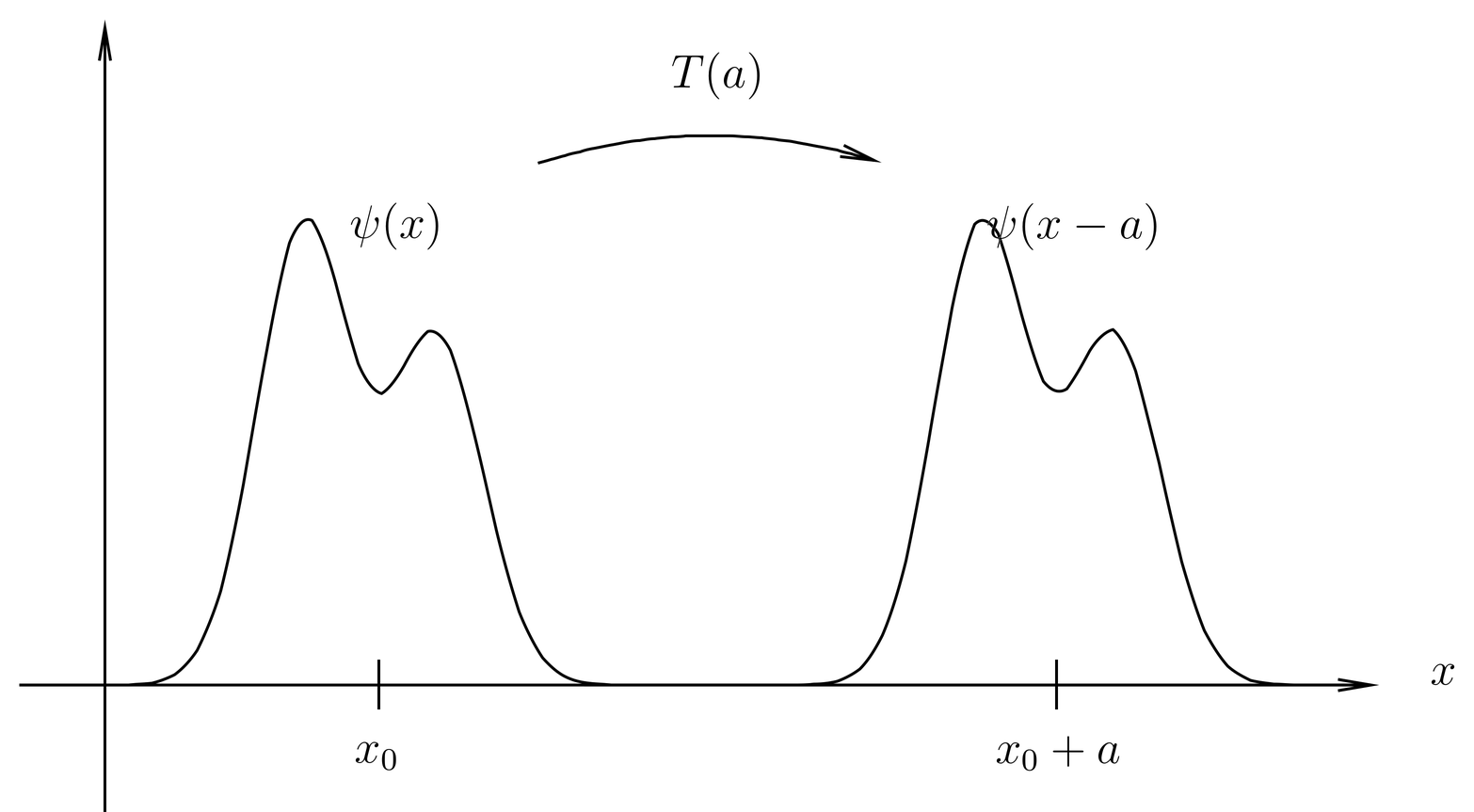
Figure 1:The action of the translation operator on a wave function .
Another remark is that that (24) uses the translation operator in a different sense from its original definition, because it is acting on a configuration space wave function instead of a ket . As we say, (24) gives the representation of the operator on configuration space wave functions.
Finally, we remark that many books would write (24) without the parentheses, that is, as
The problem with this notation is that it is not clear what acts on. is a function, and is the value of that function at a point , that is, it is a number. Does act on the function or the value of the function? Obviously, it acts on the function, which is what the extra parentheses in (24) make explicit.
The translation operator is easily generalized to three dimensions, where the displacement is a vector, and the translation operator is defined by
The other formulas and results of this are easily generalized to the three-dimensional case.
Properties of the Translation Operators
The translation operators in one dimension satisfy the following properties:
Property (27) follows immediately from the definition (21). Property (28) is the composition law that is also obvious from the definition (21); it can be proved explicitly by writing
Note that the parameter of the ket is just a label of the ket, so these labels obey the usual (commutative) rules for addition. This implies that the translation operators are commutative, as indicated in (28). The third property (29) is proved by setting in (28). The translation operators are invertible. The last property (30) states that the translation operators are unitary. We prove this by letting be an arbitrary wave function, and , so that . Then
as we prove by substituting in the middle integral. Thus, preserves the norm of arbitrary states. But a linear operator that does this is necessarily unitary (see Prob. Paragraph(c)).
Altogether, properties (27)--(30) qualify the set of translation operators as a group of unitary operators. Unitary operators appear frequently in symmetry operations because these are the only linear operators that preserve probabilities (hence, the results of physical measurements). In this case, the group is Abelian, which means that the translation operators commute with one another (property (28)).
The Generator of Translations
A simple idea that arises in the case of continuous symmetries is that a given, finite symmetry operation can be built up as a composition of smaller symmetry operations. For example, a displacement of one meter is the composition of a thousand displacements of one millimeter. In the limit we can imagine a finite symmetry operation as being built up out of an infinite number of infinitesimal symmetry operations. For this reason, special attention is attached to infinitesimal symmetry operations. It turns out that infinitesimal versions of unitary symmetry operators in quantum mechanics are always expressible in terms of certain Hermitian operators, which are called the generators of the symmetry. We will now see how this works out in the case of translations.
Thinking of a small displacement , we expand the translation operator in a Taylor series in powers of . This series begins with
The first (zeroth order) term is , and as for the second (first order) term, we notice that does not depend on so it is some operator with no parameters. We put this into a more convenient form by defining
where the hat emphasizes that is an operator (in contrast to , which is a number).
In these notes we frequently use a hat to distinguish an operator from an ordinary number, or from the classical counterpart of the operator. We normally omit the hat when there is no danger of confusion (for example, above is an operator, but we put no hat on it). But we also use the hat for unit vectors, and certain other purposes. We will explain these as they arise, so the meaning will be clear in any particular context.
Through first order, we can write the expansion of the translation operator as
We have split off a factor of in the definition (34) so that will be Hermitian. This follows when we use (35) to write out the series for and :
which by (29) and (30) must be equal. But this implies
The Hermitian operator appears in the first correction term in (35), which, when is small, is an infinitesimal translation. For this reason is regarded as the generator of translations in one dimension. That is, if we knew how to act on states with the operator , we could bring about an infinitesimal translation; and finite translations are compositions of a large number of small translations. As yet we have no physical interpretation for , but since it is Hermitian it must correspond to the measurement of some physical quantity. We will see in a moment what that is.
Exponential Form for Translation Operators
We have only written out the first two terms in the Taylor series (35) for , but the entire series can be summed and put into a neat form. To do this we will obtain a differential equation for and then solve it. See Prob. Paragraph(a), which uses similar techniques. We first write out the definition of the derivative of as a limit,
By (28), the first term in the numerator can be written as , which allows the operator to be factored out of the entire numerator to the right:
But the remaining limit is just the derivative evaluated at , which by (34) is . Altogether, we obtain
This is a differential equation that we must solve subject to the initial conditions . The solution is immediate,
Now we can easily extend the power series (35) to higher order,
We see that the generator of translations , which first appeared in infinitesimal translation operators, also appears in the exponential form for finite translation operators.
There is another way to obtain (41) that is closer to the idea of building up finite transformations from infinitesimal ones. Suppose is a displacement that is not small. We break it up into a large number of small displacements, writing . Then property (28) implies
But if is small, we can approximate by the first two terms of the Taylor series, as in (35), without assuming at this point that we know what the higher order terms are. Thus we have
This approximation should get better as gets smaller, that is, as increases. This makes it plausible that we should have the limit,
This is similar to the limit of elementary calculus,
Applying this to (45) we obtain the exponential expression (41).
Action of on Kets and Wave Functions
It is easy to work out the action of on the basis kets . We simply write
The derivative of the ket may look strange. In wave function language it is the derivative of a -function. One can use expressions with derivatives of kets as in (47), formally integrating by parts as if they were ordinary functions, and obtain correct answers.
We obtain an equivalent result that looks more familiar by working out the action of on a wave function. The procedure is the same:
We start to see the appearance of the usual momentum operator on wave functions.
Translations in Three Dimensions, and Commutation Relations
In a similar manner, for translation operators in three dimensions we define
where . This gives us a Hermitian vector operator (that is, a vector of Hermitian operators) , with components , . Now the exponential form of the translation operator is
This series can be used to obtain the commutation relations of the operators . We expand the product in power series, carrying everything to second order,
But since , the answer must be the same if we swap and . Most of the series is obviously symmetric in and , but the one term is not. When we subtract the swapped series from the original series, we obtain a vanishing commutator,
Since this is true for all choices of and , we can choose each of these vectors to be one of the unit vectors along the coordinate axes (nine choices in all), and we find
We see that is a vector of commuting, Hermitian operators.
The relations (47) and (48) are also easily generalized to three dimensions. These give
and
or, in vector notation,
(56) provides another way to derive the commutation relations (54), that is, the derivatives and commute with one another.
It is also easy to work out the commutation relations among the operators and . We just apply them to a wave function in opposite orders, obtaining
Subtracting these, we find
Combined with (11) and (54), this gives a complete set of commutation relations among the components of the operators and .
The Momentum in Classical Mechanics
We shall make a few remarks about the momentum in classical mechanics, in preparation for our discussion of the momentum in quantum mechanics.
As explained in The Momentum, there is more than one definition of the momentum of particle in classical mechanics. One is the kinetic momentum,
and the other is the canonical momentum,
where is the Lagrangian. In the case of a particle of charge moving in static electric and magnetic fields and , the Lagrangian is
so the canonical momentum is given by (35), reproduced here,
In the presence of a magnetic field (more precisely, in the presence of a vector potential) the definitions of the classical momentum (60) and (61) are not the same. We have not defined the momentum operator in quantum mechanics yet, but before we do, we must ask which of these two classical momenta will it correspond to, the kinetic or the canonical?
We have been developing the properties of the operator in quantum mechanics, which is the generator of displacements. It turns out that there is a similar role played by the momentum in classical mechanics, but it is the canonical momentum, not the kinetic, that does this. Let us write be a function of the position and momentum for a particle moving in one dimension. We can think of as a classical observable. Then we can define a classical translation operator that acts on classical observables according to
This operator moves the function forward in while leaving alone. If now is a small displacement, then the result can be expanded to first order,
But the correction term can be written in terms of a Poisson bracket of with the momentum,
Finite displacements can be built up by composing infinitesimal displacements, and the result can be expressed in terms of an exponential series of iterated Poisson brackets. We introduce the following notation for the Poisson bracket,
where and are arbitrary classical observables. Then a finite displacement can be expressed as
that is,
which may be compared to (41) and (42). The result is the Taylor series expansion of in the variable . It may also be compared to the exponential series developed in Prob. Paragraph(a).
These results are easily generalized to three dimensions. In three dimensions, the distinction between the kinetic and canonical momentum becomes important. It is the canonical momentum, not the kinetic, that generates translations in classical mechanics (in cases where it makes a difference). That is, the Poisson brackets are computed with respect to the canonical momentum, not the kinetic. See (100).
The role that momentum plays in classical mechanics as the generator of displacements is closely connected with the conservation of momentum in systems with translational symmetry. This conservation law is a special case of Noether’s theorem, which presents a general relationship between continuous symmetries and conserved quantities.
The Momentum in Quantum Mechanics
Let us work in three dimensions. According to the postulates of quantum mechanics, measurements of the momentum of a particle must correspond to some operator (actually, a vector of three operators), call it , where the hat distinguishes the classical or -number momentum from the operator. At this point we know what the Hilbert space is for particles moving in three dimensions; it is a ket space that isomorphic to the space of wave functions . But what does the momentum operator do to states in this space? That is, what is the momentum operator explicitly?
The operator is the generator of displacements in quantum mechanics, since by (35) it provides the small correction necessary when an infinitesimal displacement is carried out. Also, as noted, corresponds to the measurement of some physical quantity, and both and (the latter being the generator of translations in classical mechanics) are vectors. So the suspicion arises that is related to the momentum operator in quantum mechanics. The vector operators and cannot be equal, however, because they have different units: has units of inverse length, and has units of momentum. To make the units come out right we guess that there is a proportionality factor between and with units of action, a constant that we call :
We take this as the definition of momentum in quantum mechanics.
The postulates of quantum mechanics do not tell us what quantum operator corresponds to a given classical quantity, so we must not think that the definition of momentum is engraved in stone. The best we can do is to find a vector of operators in quantum mechanics that has properties similar to the classical momentum and that goes over to the classical momentum in the classical limit. In fact, the similarity with the classical momentum (as the generator of translations) has motivated the definition (70), and, as for the classical limit and the other expected properties of momentum, they will be laid bare as we proceed.
The Constant 
Notice that did not appear in the postulates of quantum mechanics; it appears for the first time in our development of the formalism in (70). The value of in ordinary units must be determined experimentally. The discussion so far has been based on the analysis of a single particle moving in three-dimensional space, so one might question whether different particles have different values of . We would not get the usual classical limit if this were so, so it seems theoretically doubtful that there are different values of , but it is a question that can be tested experimentally (all the ’s turn out to be the same to within experimental accuracy). Given that there is only one , there is the option of choosing “natural units” in which .
The relation (70) implies the usual de~Broglie relation connecting momentum and wavelength,
as we shall show momentarily, so the value of can be determined by measuring the de~Broglie wavelength of a particle of a known momentum. The most elegant experiments along these lines have involved Bragg diffraction of a neutron beam from a single, large (about 10cm) silicon crystal with no dislocations or grain boundaries. The manufacture of such crystals has become feasible with modern semiconductor technology. The predictions of the relation (70) are fully confirmed. Actually, if (70) were not correct, there are very few of the theoretical predictions of quantum mechanics that would agree with experiment.
The silicon neutron interferometer just mentioned was used in the 1970’s to measure the phase shift of neutron wave functions as the neutrons fall in the earth’s gravitational field. This was the first demonstration that gravitational potentials enter the Schr"odinger equation in the same manner as other potentials. The experiment and results are discussed in Sakurai, Modern Quantum Mechanics and in Commins, Quantum Mechanics: An Experimentalist’s Approach. Commins has a particulary nice explanation of the neutron interferometer.
The fact that is a universal constant was known to Planck and others in the 1890’s, even before quantum mechanics existed. Planck knew that a constant with dimensions of action must occur in the expression for the spectrum of black body radiation, even before the correct expression was known. He also realized that , and (Newton’s constant of gravitation) could be combined to create a natural system of units for distance, time and mass. The Planck unit of distance is
It is the length scale at which the effects of both quantum mechanics and gravity are expected to be important. Physics at such scales is currently a matter of much speculation, and is likely to remain so for some time, in view of the near impossibility of direct experimental tests. Nevertheless the importance of the length scale itself has been known for a long time.
The Momentum in Quantum Mechanics: The History
The pseudo-axiomatic approach we are taking here to the development of the momentum operator in quantum mechanics is quite different from the historical one. In a series of papers between 1905 and 1916, Einstein developed the idea that light of frequency and wave vector is associated with particles of energy and momentum . We now call these particles “photons,” although that name was not coined until later. According to Maxwell’s equations the frequency and wave number of a light wave are related by , so Einstein’s formulas give the energy-momentum relation for the photon as , exactly what the special theory of relativity predicts for a massless particle traveling at the speed of light. Einstein’s arguments relied heavily on statistical mechanics. Most physicists of the time regarded the idea of particles of light as completely crazy, since it had been established a hundred years earlier that light was a wave. But in 1922 Compton showed experimentally that collisions between x-rays and electrons obey the relativistic rules of conservation of energy and momentum, assuming Einstein’s expressions for the energy and momentum of the photon. With this physicists began to take the wave-particle duality more seriously. In 1924, de~Broglie argued that if light could have both wave and particle aspects, then so might ordinary particles also have wave aspects. This was in part an appeal to the unity of physics, and a suggestion offered by the equivalence of energy and mass, as shown by special relativity. De~Broglie suggested that the formulas and should apply also to massive particles, giving the frequency and wave vector of a wave associated with the particles. Somewhat later Debye remarked that if there was a wave, there should be a wave equation, and Schr"odinger, on hearing of this, set out to find it. He first tried a relativistic wave equation without success, only later trying the nonrelativistic version which gave an explanation of the hydrogen spectra and other physical facts. The latter equation is the one usually associated with his name.
A good recent book that covers this history and much else is Einstein and the Quantum by A. Douglas Stone.
Properties of the Momentum
We will provisionally accept the definition (70) of the momentum operator in quantum mechanics, and proceed to examine the consequences. First, the translation operators can now be written in the form,
The various commutation relations we have evaluated may now be expressed in terms of instead of and gathered together in one place,
These are the Heisenberg-Born commutation relations. They may be compared to the classical canonical Poisson bracket relations, (108).
Also, the properties (55) and (57) of the operators are easily translated into the properties of the momentum. We have
and
(77) gives the action of the momentum operator in ket language, whereas (78) gives it in the position representation. It has other forms in other representations. Another form of these equations is
This is really a rephrasing of (78), and can be obtained by taking the Hermitian conjugate of (77) and then multiplying by the ket .
The Momentum Representation
Because is a vector of commuting, Hermitian operators, these operators possess a simultaneous eigenbasis. We write the eigenvalue-eigenket problem for momentum in the form,
We solve this in the configuration representation, that is, we multiply (80) on the left by the bra , define the wave function of the momentum eigenket by
and use (78) to obtain
Thus, is the eigenfunction of the differential operator (really three commuting differential operators) with eigenvalue . The solution exists for all values of and is unique to within a constant,
where is a normalization and a phase. Thus, momentum has a continuous spectrum, so we normalize the eigenstates according to
Using the integral
the normalization constant in (83) is determined to within a phase, which we fix by demanding that be real and positive. The result is
The eigenfunctions of momentum are plane waves, whose wave length is given by the de~Broglie relation (71).
Since the momentum eigenstates are nondegenerate, the momentum operators form a complete set of commuting observables, and we may speak of the momentum representation. The resolution of the identity in this representation is
We will denote the wave function of the state in the momentum representation by
(compare (15) for the configuration representation), so that by multiplying (87) onto the ket we obtain
similar to (16) in the configuration representation. The wave function is the expansion coefficients of the state with respect to the momentum eigenbasis .
By using (86) and resolutions of the identity it is easy to switch back and forth between wave functions and , representing the same quantum state in two different representations. For example, we have
and its inverse,
The wave functions and are Fourier transforms of one another, modulo the insertion of factors of to account for the physical units.
In the momentum representation, the operator is represented simply by multiplication by , the vector of -numbers. That is, if is given in terms of the state by (88), then the momentum space wave function of the state is
where we have allowed to act to the left on the bra , bringing out the eigenvalue . We can write this as
Similarly, the operator in the momentum representation is given by
Compare this to (78), and notice the difference in sign. This follows since if is related to by (88), then what we mean by the left-hand side of (94) is
Finally, we summarize the representations of the operators and in the configuration and momentum representations in Table 1.
Table 1:Representations of the operators and when acting on configuration and momentum space wave functions. \par
Configuration | - | |
Momentum |
Multiparticle Wave Functions
In a system of particles, the positions of the individual particles are independent observables that commute with one another, so a complete set (ignoring spin for now) consists of the operators , with eigenvalues . In this case the wave function is defined by
The wave function is defined over configuration space, that is, the space in which a single point specifies the positions of all the particles. This is the same configuration space as in classical mechanics, which is discussed in Constrained Systems, Configuration Space, and Generalized Coordinates. Configuration space coincides with physical space only in the case of a single particle. Similarly, one can define a multiparticle, momentum space wave function .
If one is careful about the application of the postulates of quantum mechanics, one will see certain subtleties in the derivation of (97) in the case of identical particles. We will examine this question more carefully in 29. Identical Particles.
The Sign of 
The following is a remark concerning the the definition of in (34), which led to the definition of momentum in (70). We split off a factor of in (34) to make Hermitian, but the same would have been achieved if we had split off (thereby changing the definition of by a sign). This would lead to the opposite sign in the definition of , and changes in signs in many of the subsequent formulas. Would this change lead to any physical consequences or contradictions with experiment?
The answer is no, but it would change most of the familiar formulas in quantum mechanics, by replacing by . For example, a plane wave with wave vector would become instead of the usual . It is a matter of convention to choose the sign of in quantum mechanics, and our choice has been made in (34) and (70). Once this choice has been made, however, then the sign of the Pauli matrix is determined, so that spin angular momentum has the same commutation relations as orbital angular momentum. This was a question addressed in Prob. Paragraph(d).
The Position-Momentum Uncertainty Relation
The generalized uncertainty relations (53), applied to the case of position and momentum of a particle in one-dimension, for which , give
This can be used in a number of applications to obtain quick estimates of orders of magnitude of physical quantities, including three-dimensional problems where for simplicity we ignore the vector nature of and . We give several examples.
Consider a beam of particles of well defined momentum directed at a screen in the plane . The screen has a hole of dimension (the hole need not be circular, is just an order of magnitude estimate of the size of the hole). The hole confines the particles in the - and -directions to a distance of order , so by (98) the particles acquire a transverse momentum (in the - or -directions) roughly of magnitude
where we drop constants of order unity since this is only an estimate. Thus downstream from the hole the beam should spread at an angle given roughly by
where is the wave length of the incident waves. This calculation assumes the angle is small, which is equivalent to , that is, the hole should be at least a few wavelengths in diameter. This very simple estimate of the spreading angle of the beam is confirmed by more complicated calculations of diffraction theory in the far-field (Fraunhofer) region.
If we eliminate all momenta in favor of wave numbers , by , then all the ’s disappear and we have results that can be applied also to classical waves (light waves, sound waves, etc).
For another example, let be an estimate of the size of a hydrogen atom. The electron is confined to a distance of order and so must have a momentum of order . In a circular orbit this implies a centrifugal force of
Equating this to the electrostatic force on the electron from the proton, , and solving for , we obtain
This is the usual expression for the Bohr radius. Given an estimate for the size of an atom and the known density of ordinary matter, one also obtains an estimate for the Avogadro number and many other physical quantities.
Minimum Uncertainty Wave Packets
Let us loosely define a wave packet in one dimension as a wave function whose dispersions and , defined as in Statistical Aspects of Measurement by
are small, that is, close to the minimum values allowed by the inequality,
See (54). Similarly, let us define a minimum uncertainty wave packet as one for which the product takes on its minimum value of .
Let be a normalized, minimum uncertainty wave packet with
and let , so that . Now let
The operator appearing on the right seems to have been pulled out of the air, but it is a version of an annihilation operator of the general form , with coefficients adjusted to make the following argument come out right. We will see such annihilation operators again when we discuss the harmonic oscillator. Now squaring (106), we obtain
This implies (see (28), so (106) in wave function language becomes
which has the normalized solution,
The minimum uncertainty wave packet is a Gaussian. If we allow and to take on arbitrary values , as shown, then we find
where is a phase. The wave packet is still a Gaussian, but it has been shifted in position and momentum.
Problems
Problem 1.
Let be the state of a spinless particle in three dimensions, and let be its momentum space wave function. Find the momentum space wave function of the state , that is, find the action of the translation operator in the momentum representation.
Problem 2.
Consider a particle moving in one dimension. In classical mechanics, the state of the particle is given by its position and momentum , and other observables such as energy are functions of these. The classical position and momentum are ordinary numbers, and obey the usual (commutative) rules of algebra, for example, . In quantum mechanics, we have the operators and which are analogous to the classical and , and other observables such as the Hamiltonian are functions of and . On the other hand, and do not obey a commutative algebra, in view of the relation .
A question that has exercised various people is the relation between classical observables (that is, functions of } and ) and quantum observables (that is, functions of and ). One problem is to quantize a classical observable, that is, given a classical function , what is the corresponding quantum observable? Dirac suggested that and should be associated with and , but this gives rise to an ambiguity in cases like the classical function . Should it correspond to or to , or maybe to their average (which at least would be Hermitian)?
Another answer to this question was given by Weyl. We introduce the Weyl transform in this problem because it is good exercise in the position and momentum representations.
We denote operators with a hat, as in or , and we denote eigenvalues or classical quantities without a hat, as in or . We work in one dimension, and think of a wave function or .
If is an operator, we define the {\sl Weyl transform} of , denoted , by
Here the notation , for example, means the eigenket of with eigenvalue . It is useful to think of as a function defined on the classical phase space which is in some sense the classical observable corresponding to the quantum operator .
(a) Show that if is the Weyl transform of operator , then is the Weyl transform of . In particular, this shows that the Weyl transform of a Hermitian operator is a real function on phase space.
(b) Show that if operators and have Weyl transforms and , respectively, then
Notice how the right hand side looks like the “scalar product” of two classical observables on phase space.
(c) Find the Weyl transforms of the following operators: 1 (the identity operator); ; ; ; ; .
(d) The classical probability density in phase space (see Classical Statistical Mechanics) describes a system whose dynamical state can only be described statistically. Since is a probability density, it is nonnegative, , and it is normalized,
The probability density in alone (call it ) or in alone (call it ) is obtained by integrating over the other variable ( or ),
and each of these is normalized,
The functions or are called marginal distributions in statistics.
It turns out that the Weyl transform of the density operator in quantum mechanics is very similar in its properties to the classical probability density . The function is called the Wigner function. Because is Hermitian, the Wigner function is real.
For simplicity let us work with a pure state, so . Express the marginal distribution
in terms of the wave function . Now let be the momentum space wave function, and express the marginal distribution
in terms of . What is the normalization integral,
These results suggest that is a distribution function of particles in phase space whose statistics reproduces the statistics inherent in quantum measurement, apart from the normalization. Unlike a classical distribution function , however, can take on negative values. These “negative probabilities” have no meaning in any statistical sense, but they only arise, in a certain sense, when we attempt to measure and simultaneously to a precision greater than that allowed by the uncertainty principle. The Wigner function can be used to express quantum statistical mechanics in a manner that is surprisingly similar to classical statistical mechanics, but one which is still fully quantum mechanical.
Problem 3.
Given that the range of the nuclear forces is approximately 10-13~cm, estimate the velocity of the proton or neutron in a deuteron (a bound state of a proton and a neutron). Compare this to the of the electron in the ground state of hydrogen. It is believed that nuclear forces are independent of the charge state of the nucleon; thus, two protons should feel the same nuclear force as two neutrons. Calculate the nuclear force between two protons at a distance of 10-13~cm and compare to the electrostatic force.
Problem 4.
Let be an arbitrary function of and and arbitrary function of . Evaluate the commutators, and .
Problem 5.
The Large Hadron Collider is designed to reach an energy of 7~TeV (~eV). What is the smallest distance scale that can be probed at these energies? How does it compare to the Planck length, at which the effects of quantum gravity are expected to be important?