03. The Density Operator
The Quantum State of a Thermal Beam
Consider the apparatus illustrated in Figure 1. A collimated beam of silver atoms is extracted from an oven, which is then passed to observer~1, who with a Stern-Gerlach apparatus measures . In these notes we will speak of measuring spin instead of magnetic moment; these are proportional,
so measuring one implies the measurement of the other. (But physically the Stern-Gerlach apparatus really measures magnetic moment.) Of the two beams that emerge from the apparatus, the one with measured value is thrown away.
In the previous set of notes we decided that the Hilbert space for the spin of a silver atom is two-dimensional, and that the eigenspaces of (which are the eigenspaces of ) are one-dimensional. Therefore according to the postulates of quantum mechanics, whatever the state of the beam when it enters the first apparatus, it will be projected onto the one-dimensional eigenspace of with eigenvalue when is measured. Therefore the state of the beam emerging from the first measurement apparatus is described by any nonzero vector in this eigenspace. We let be such a vector, assumed to be normalized. The beam is passed to observer~2, who measures some other observable . According to the measurement postulates of quantum mechanics, observer~2 will measure an average value of given by
The quantity is the average of a large number of measured values of observable , which are made on different silver atoms.
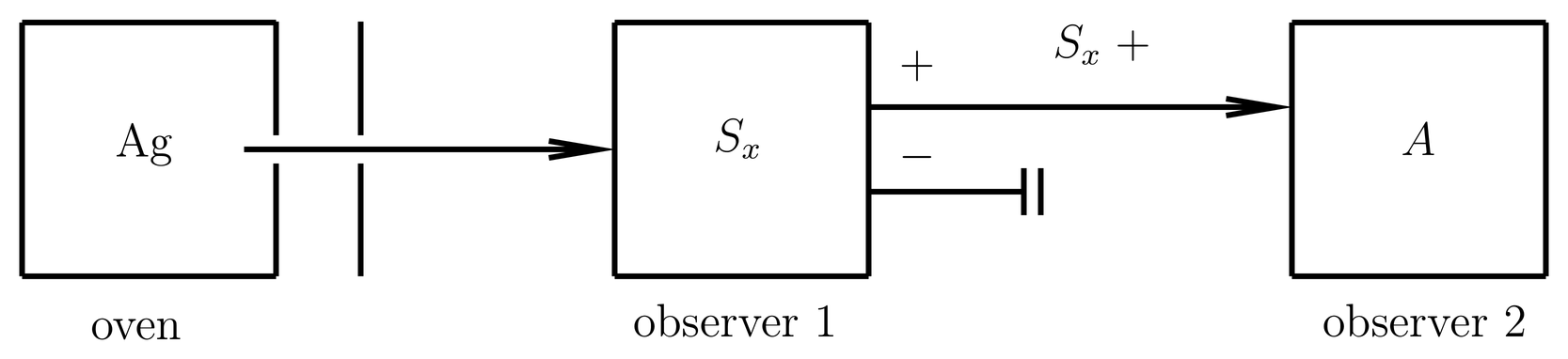
Figure 1:An atomic beam from a thermal source is prepared by observer 1 who measures , and is then passed to observer 2 who measures some observable .
Thus the quantum state of the beam emerging from the first apparatus is known. But what about the beam that enters the first apparatus, coming from the oven? How is its quantum state described? Is it also associated with some state vector?
Thermal Beam Not Described by a State Vector
The answer is definitely no, for a beam from a thermal source such as we have described is isotropic, and has no preferred direction of spin. For if we measure on the thermal beam we find 50% of the atoms with and 50% with , for an average of . Similarly we find , or . Naturally, the thermal beam has no preferred direction of spin.
On the other hand, any definite quantum state (a so-called “pure” state) of the spin system is associated with a normalized ket in the 2-dimensional Hilbert space, and such a ket is not isotropic but rather necessarily “points in” some direction. To show this, let us represent an arbitrary normalized ket in terms of its components with respect to the basis , , consisting of eigenkets of the observable . Then can be written in the form,
where
We can equally well represent in terms of a 2-component spinor,
where the column spinor contains the components of with respect to the basis . Then by using and the standard forms for the Pauli matrices , we easily find
where the vector is the real, 3-component vector shown. Vector is a unit vector, as follows immediately by computing and using (4). Thus, does not vanish, but rather points in some direction . For example, one finds that the state “points in” the direction.
Conversely, if a direction is specified by its usual spherical angles ,
then it is possible to construct a normalized spinor “pointing in” this direction; this spinor is unique up to an arbitrary overall phase. With one choice of phase convention, this spinor is given by
or,
The upshot of all this is that the state of the beam emerging from the oven cannot be described by any definite ket in the Hilbert space.
A Random Ensemble of State Vectors
Now let us modify the apparatus by allowing the first observer to orient his or her Stern-Gerlach apparatus in an arbitrary direction , as illustrated in Figure 2, to measure the component of in the direction . Furthermore, let us suppose that before each silver atom enters the first apparatus from the oven, the first observer chooses a random direction , uniformly distributed in solid angle, in which to orient the apparatus. (Fortunately, this is a gedankenexperiment, but what we describe is possible in principle. The easiest way to measure the component of the spin in an arbitrary direction would probably be to rotate the spin, rather than the magnet, before the measurement. This could be done with a uniform magnetic field. It is also possible in principle to change the direction of the beam without changing the spin by use of an inhomogeneous electric field.) The first observer keeps this information secret from the second observer, who therefore has no knowledge of the state of polarization of the beam he or she is receiving.
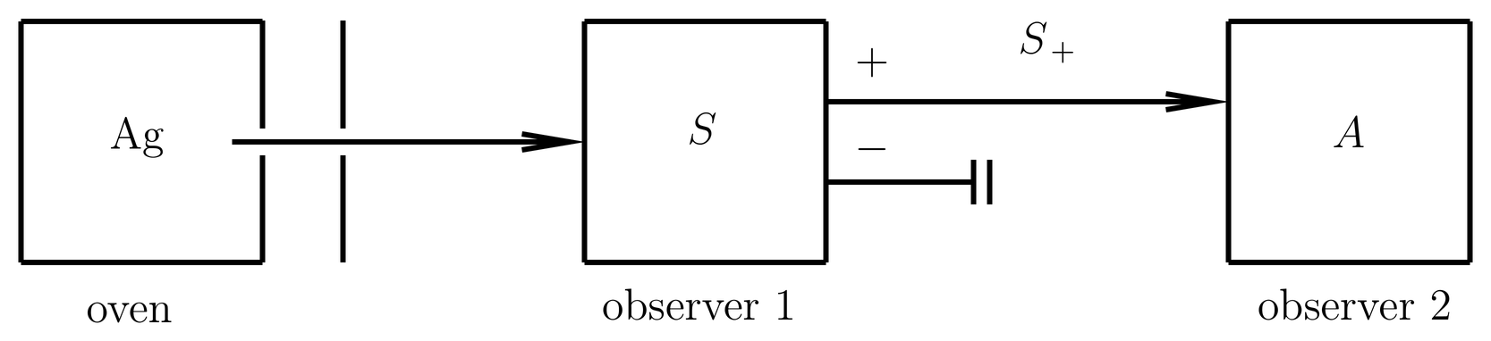
Figure 2:Now the first observer polarizes the beam in a random direction .
Under these circumstances, the second observer will be unable to tell, by any measurement performed on the beam, whether the beam has passed through a randomly oriented Stern-Gerlach apparatus on its way from the oven, as illustrated in Figure 2, or whether it has been received straight from the oven. (We assume that observer~2 has no information about the intensity of the beam, which otherwise would allow the two cases to be distinguished.) In the absence of knowledge about the orientation of the first apparatus, the two cases are physically indistinguishable.
[Of course, in making these statements, we are assuming that the beam from the oven really is unpolarized, in the sense that . It is a matter of experiment to decide whether this is true or not, and we can imagine physical processes in the oven that would result in a net polarization of the beam from the oven. For example, magnetic fields in the oven would impart an energy difference (small, but nonzero) to the two spin states, and then the Boltzmann factor would give different weights to the two states. But for the sake of this discussion, we assume that the thermal beam really is unpolarized.]
Accepting the equivalence of these two physical situations, we can write the average value of , measured on the beam taken directly from the oven, as
where represents the element of solid angle of the direction in which points, and where the integral simply averages the expectation value with respect to a definite state over all solid angles. The isotropy of the beam is achieved, not by any definite state vector, but by an isotropic probability distribution of state vectors.
Ensembles of State Vectors from a General Standpoint
Let us now consider state vectors distributed according to some probability distribution from a more general standpoint. Let be a family of normalized kets depending on some continuous parameter (or parameters) , and suppose is distributed according to some probability distribution , so that and
For example, in the situation discussed above, could be identified with the angles , so that would represent . Then the expectation value of an arbitrary operator is given by
in which the notion of expectation value includes both the statistics inherent in the measurement of a definite quantum state, and the lack of knowledge about that quantum state. The experimenter cannot tell the difference between these two types of statistics, based solely on experiments performed on the systems he or she receives.
The discrete case is also of interest. Suppose is some set of normalized kets, where is a discrete index to which probabilities are assigned, so that and
Then the expectation value of an arbitrary operator is given by
It is important to note that the kets are not assumed to be orthogonal; they simply represent a collection of states to which probabilities are assigned. Nor in the continuous case is there any orthogonality relation assumed among the kets for different values of the parameter ; for example, in the Stern-Gerlach apparatus discussed above, the states for different values of are not orthogonal unless the two vectors point in opposite directions.
The Density Operator
We now express the expectation values (12) or (14) in terms of the density operator , defined in the continuous case by
and in the discrete case by
In terms of , the expectation values (12) and (14) can be written,
as follows immediately from the definitions of and the properties of the trace. (17) is a fundamental result in quantum mechanics, as it expresses the results of an arbitrary measurement in the general case in which the state vector is only known in a statistical sense.
The generality of (17) is even greater than is apparent. At first sight is seems that the measurement of the average value of an observable is a special kind of measurement, and furthermore one that throws some information away. For example, if the measurement of produces three values, , and , with associated probabilities , , and , then when we compute the average value we have lost information about the possible outcomes and their probabilities. But that information is available if we replace by one of its projectors, say , whose average value is ; or if we replace by , whose average value is . Thus, with a sufficiently broad interpretation of the operator that appears in (17), we can say that every possible physical measurement that can be made on a physical system gives a result that can be written in the form (17). Therefore knowledge of the density operator allows one in principle to calculate the results of any measurement process.
Pure and Mixed States
The case in which the state of the system is known to be represented by a definite state vector, for example the case of the beam delivered to the second experimenter in Figure 1, is one in which one state vector can be assigned a probability of 100%, and all other state vectors have probability zero. In this case, the density operator has the form
where is the state vector in question, assumed to be normalized. In this case we speak of a pure state. On the other hand, if there is any statistical uncertainty in the state vector, then we speak of a mixed state. Mixed states are the norm in real experiments. There is some subtlety in this definition, because if we have two kets and that differ only by a phase factor, and we decide to attach 50% probability to each, then in fact we have a pure state. This of course is what we expect, since the two kets are physically equivalent. Similarly, if kets and are nearly linearly dependent, and the system is known to be in one or the other with 50% probability, then the system is nearly in a pure state. On can quantify the degree of “pureness” with the entropy, which is discussed below.
Pure and mixed states in quantum mechanics are similar in many respects to coherent and incoherent light in optics. For example, an ensemble of light waves with random phases but very nearly the same vector (all moving in nearly the same direction with the same frequency) represents nearly coherent light. This is the case with light from a star, in which the angular spread in is the very small angular diameter of the star. Although the individual light wave are emitted incoherently by atoms on the surface of the star, the light arrives at earth in a high degree of coherence. (More precisely, it has a large correlation length, which can be many meters. As realized by Michaelson, measurements of this correlation length can be used to determine the angular diameter of a star, something that cannot be done with ordinary telescopes because the angles are too small).
A Complete and Minimal Description of the Physics
The density operator contains a complete and minimal description of the information available about the given system (more precisely, about the ensemble of identically prepared systems). The description is complete because, as discussed above, knowledge of suffices to calculate the outcome of any statistical measurement. The description is minimal because can be measured (see Measuring the Density Operator). There are no phase or other conventions involved in determining the density operator. Therefore the density operator contains the physics, all the physics, and nothing but the physics. This is in contrast to wave functions or state vectors, which are subject to phase conventions (and which in any case only work for pure states). It is easy to see from the definitions (15) and (16) that the density operator is independent of the phase conventions inherent in its constituent state vectors.
The Statistical Nature of the Measurement Process
In these discussions, however, the measurement process in quantum mechanics must be understood in the appropriate, statistical sense. The postulates of quantum mechanics are obviously stated in statistical terms; nothing is said about the outcome of a measurement performed on an individual system. For example, if we feed a -polarized beam of silver atoms into a Stern-Gerlach magnet oriented in the -direction, then neither quantum mechanics nor anything else in the universe can say whether an individual silver atom will go up or down in the magnet. What quantum mechanics does do is make predictions about the distribution of up- and down-going atoms when large numbers of silver atoms, prepared in an identical way, are sent into the -magnet. In the general case, we must imagine an ensemble of identically prepared systems---in imagination, an infinite number---upon which measurements are made. Quantum mechanics predicts the statistical distribution of measurements on such ensembles. In the orthodox interpretation of quantum mechanics, that is all it does: the density operator , which is measurable on an ensemble of identically prepared systems, is the repository of all information about that ensemble of systems, and allows us to predict the outcome (in a statistical sense) of any experiments performed on that system in accordance with (17).
Quantum Statistics and Hidden Variables
In quantum mechanics it is meaningful to talk about the value of a certain observable, if the system has been prepared in an eigenstate of that observable with some eigenvalue (which is done by measuring that observable and keeping only those systems with a particular outcome). Then subsequent measurements of that observable will return the given eigenvalue with 100% probability, as explained in Statistical Aspects of Measurement. More generally, we can prepare a system in a simultaneous eigenstate of commuting observables, and we can talk about the values of those observables. If the observables in question are not constant in time (if they do not commute with the Hamiltonian), then the system will not remain in the given eigenstate, and in order to obtain the 100% probability quoted it will be necessary to make the subsequent measurements immediately after the preparation. In particular, the Hamiltonian for an isolated system commutes with itself, so if a system is measured to have a certain energy, then it is meaningful afterwards (assuming the system remains isolated) to talk about its energy.
There is, however, no role played in the orthodox interpretation of quantum mechanics for the simultaneous values of noncommuting observables. These are in principle not measurable. We are of course tempted by the analogy with classical mechanics to think in such terms, because in classical mechanics such simultaneous values of noncommuting observables are meaningful. But to do so means that we are using concepts for understanding physical reality that have no physical consequences. One is reminded of Newton’s ideas of absolute space and time, which likewise had no physical consequences, and which were eliminated from physics with the advent of relativity theory. The idea of basing quantum mechanics on strictly measurable quantities seems to be due to Heisenberg, who was apparently influenced by Einstein’s similar reasoning in his development of relativity theory.
In classical statistics, we can reduce our uncertainty about an ensemble (increase our information) by filtering the system, for example, extracting balls from an urn and keeping only those with a red spot. The new (reduced) ensemble is now known to contain only balls with a red spot on them. Similarly, in quantum mechanics, we can reduce our uncertainty of a system described by some density operator by performing measurements. As discussed later in these notes, a measurement produces a new density operator , representing a (reduced) ensemble about which we have more information. Our information (or rather the lack of it) can be quantified by the entropy, defined in (37), which reaches its minimum value of zero when a complete set of commuting observables has been measured and the system is in a pure state. Even in a pure state, however, the results of experiments are still predicted only in a statistical sense. In this important sense quantum statistics differs greatly from classical statistics.
The idea that nature is intrinsically statistical is one that has not sat well with a number of physicists, notably Einstein. One way of escaping from the orthodox view is to imagine that there are extra dynamical variables present in a physical system, so-called “hidden variables,” which we do not usually measure but which, if we could know them, would allow us to predict the outcomes of individual measurements. There are a variety of hidden variable theories that compete with quantum mechanics and attempt to explain the experimental results within a framework that is fundamentally deterministic, not statistical. These theories can be classified as “local” or “nonlocal.” In a nonlocal hidden variable theory, communication between different parts of the system takes place faster than the speed of light, that is, instantaneously in some Lorentz frame. Since this seems unlikely from the standpoint of relativity theory, local hidden variable theories seem preferable. However, as first shown by J. S. Bell in 1965, local hidden variable theories give physical predictions that differ from those of quantum mechanics. Experiments testing these predictions were carried out by Alain Aspect in the 1980’s, and they showed that quantum mechanics is correct. For this reason, there does not seem to be much room left for hidden variable theories, although there is speculation about nonlocal hidden variable theories in quantum gravity. See Quantum Gravity by Lee Smolin for a nontechnical discussion of some of these ideas.
For these reasons it seems to me that the orthodox view of quantum mechanics is probably correct, and that it is unwise in talking about quantum mechanics to use a language that implies a reality to the simultaneous values of noncommuting observables. I suspect, however, that there will be a reinterpretation of quantum mechanics when and if quantum gravity is finally comprehended.
The Properties of the Density Operator
We return now to the density operator and describe its characteristic properties, of which there are three. First, is Hermitian, as follows immediately from the definitions (15) and (16). Second, is nonnegative definite (see (67), as follows by computing the expectation value of with respect to an arbitrary ket ,
where for simplicity we work with the discrete case. The third characteristic property of a density operator is that it has unit trace,
This property is equivalent to the normalization condition on the probabilities, (11) or (13), as one can easily show. Conversely, as we shall show below, every nonnegative definite, Hermitian operator with unit trace can be interpreted as a density operator, that is, there exist kets and corresponding statistical weights such that the operator can be written in the form (15) or (16).
Decomposing a Density Operator into Pure States with Weights
Let us return now to the atomic beam emerging from the oven in Figure 1 or Figure 2, and actually compute the density operator that represents it. We use the continuum formula (15), which in the present case becomes
We write the integrand in terms of spinors and matrices in the basis, so that the outer product becomes the product of a column spinor times a row spinor,
Here we are identifying with the state in (9). When we average the resulting matrix over solid angles, the off-diagonal elements vanish, and the diagonal elements each give . Therefore is represented by a multiple of the identity matrix in the basis,
or, in terms of explicit basis vectors,
Although this calculation was carried out in the basis, the answer is independent of that basis. It is an important lesson of this calculation that an isotropic density operator is represented by a multiple of the identity matrix; as we will see later when we discuss the theory of rotation operators, only such a matrix is invariant under rotations.
Let us now return to the apparatus sketched in Figure 2, and change the game somewhat. Let us suppose that observer~1, instead of choosing the orientation of the Stern-Gerlach apparatus uniformly over all solid angles, makes a choice between only two possibilities, and , each with probability. That is, suppose the only two directions chosen for lie at the north and south poles. Then we have an example of a discrete set of state vectors as in (16), with identified with and for , each with probability . It follows that the density operator is
But this is the same density operator as in (24), obtained under the assumption of an isotropic distribution of vectors ! Therefore, since the density operator contains within it the results of all physical measurements that can be performed on the ensemble of systems, it is impossible to tell by any experiment whether the ensemble contains atoms polarized in directions that are random and uniform distributed over all solid angles, or simply in the directions.
The “Real” Wave Functions
There is another important lesson contained in this result, namely, that there is no unique decomposition of a given density operator into a set of pure states with probability weights. Such a decomposition into pure states and associated weights can be carried out in many different ways. But since the density operator contains all the physics that can be measured on a given ensemble of systems, one cannot determine by any physical measurement which pure states and associated weights are the “real” ones. The reality is the density operator itself.
This point would be easier to understand if we had not defined the density operator in the first place in terms of pure states and associated weights [(15) and (16)]. We did this because you have probably spent more time thinking about wave functions than density operators, so you have some feel or intuition for wave functions. Mixed states may be the norm in real experiments, but pure states are the norm in first courses in quantum mechanics and homework problems. But our presentation has been circular: we defined the density operator in terms of pure states, and then defined a pure state in terms of the density operator. A more satisfactory approach would be to incorporate density operators into the postulates of quantum mechanics from the outset, and then to “derive” pure states as a special case. We will, in fact, present a revised and final version of the postulates of quantum mechanics in The Postulates of Quantum Mechanics (Revised), formulated in terms of the density operator, and you should regard these as a satisfactory starting point for understanding the measurement process in quantum mechanics.
This point has interesting implications in some practical situations. Consider, for example, a scattering experiment, in which a beam of particles is directed at a target. As you know, in mathematical treatments of scattering theory, it is common to speak of a plane wave incident on a target, which is scattered into a scattered wave. This is done for reasons of mathematical simplicity, but note that a plane wave is not normalizable and cannot represent the quantum state of a real particle. A more sophisticated approach uses wave packets, which is somewhat closer to real physics because wave packets are normalizable and can represent physically realizable states (but pure ones). But when we are faced with a real accelerator, an obvious question is, what actually is the wave function of the particles coming out? Is it a plane wave, a wave packet, or something else? And how would we know? The answer is that in most cases the state of the particles emerging from an accelerator is not a pure state at all, but rather a statistical mixture, which must be represented by a density operator. Since the density operator has no unique decomposition into pure states, the question about the “real” wave function of the particles is meaningless.
Another shortcoming in first courses in quantum mechanics is that they spend a lot of time talking about wave functions, but little time explaining how a wave function is measured. Measuring a wave function in quantum mechanics is not like measuring a wave field in classical mechanics (for example, an electromagnetic wave). Consider, for example, a spinless particle moving in three dimensions. As you know, if the system is described by a wave function , then the probability density for finding the particle somewhere is space is
Certainly we can measure , at least in principle, by making measurements on an ensemble of identically prepared systems. And if the system is described by a wave function , then we have determined the amplitude of , that is,
where is a phase that is not determined by our measurements and which may be a function of position. Obviously further measurements are needed to determine this phase.
But before we do that we must ask, how do we even know that the system is represented by a wave function , that is, how do we know that it is in a pure state? If the system is represented by a density operator that has a decomposition into a discrete set of pure states and associated weights as in (16), then what we have actually measured is
This in fact is the diagonal matrix element of the density operator in the position representation,
that is, we have measured
The -space matrix elements of given in (29) actually constitute the correlation function of the quantum wave function. Generally speaking, the correlation function of a wave field is the statistical average of a product like , for example, one can talk about the correlation function of the electric field in optics. Thus, before we attempt to measure the phase in (27), we should make sure that we have a pure state. One way to do this would be to measure the off-diagonal elements of , thereby determining as an operator, and then decide whether it represents a pure state. See Criteria for a Pure State.
General Properties of the Density Operator (Continued)
In the following (and for the rest of the course) we will adopt the point of view that the density operator is the primary object and that pure states are just a special case. This is certainly how it is in real experiments, but it means that our original “definitions” of the density operator, in (15) and (16), are not satisfactory, because they express the density operator in terms of a statistical ensemble of pure states. Nevertheless, those equations do give a useful perspective on the density operator, which is directly applicable in situations such as the gedankenexperiment we considered earlier in which the beam of atoms was polarized in a random direction. Moreover, as shown in The Properties of the Density Operator, they lead to three important properties of the density operator: it is Hermitian, it is nonnegative definite, and it has unit trace.
To pursue this idea, we now ask, if an operator has these three properties, can it be represented as a statistical mixture of pure states? That is, do there exist weights and state vectors such that (15) or (16) is true? The answer is yes, as we now show.
Suppose we have a nonnegative definite, Hermitian operator of unit trace. Consider its eigenkets and eigenvalues ,
The operator can only have a discrete spectrum, because any operator with a continuous spectrum has a trace that is infinite (or not defined, see \hilbert.22). Since is Hermitian, the eigenvalues are real. Furthermore, since is nonnegative definite, we can multiply (31) on the left by to obtain
Next, by summing this over and using the fact that , we obtain
so that the are nonnegative numbers that sum to unity and can be interpreted as probabilities. Finally, expressing in terms of its eigenvalues and projectors, we have
which is a special case of (16). This proves the assertion.
We see that an arbitrary density operator can actually be represented in terms of a discrete, orthonormal set of pure states and associated weights; but we emphasize again that in the general representation of a density operator in terms of pure states, as in (16), there is no requirement that the states be orthogonal (nor do they have to belong to a discrete family, as we have seen in the example discussed in A Random Ensemble of State Vectors). We also emphasize that the decomposition of into pure states and weights is not unique. Nevertheless, since such a decomposition always exists, it is never wrong to assume such a representation of a density operator for the purpose of calculation or of understanding its properties.
Criteria for a Pure State
How do we know if a density operator is actually a pure state, that is, that it can be written for some normalized ket ? The most direct answer is to diagonalize . If all the eigenvalues are zero except one that is 1, and if the eigenvalue 1 is nondegenerate, then the state is pure, and it is represented by the eigenket of with eigenvalue 1. It that case is a projection operator onto the one-dimensional eigenspace of eigenvalue 1.
Here are some other criteria for a pure state. First we have the theorem, that for any density operator ,
with equality if and only if represents a pure state. The proof of this theorem will be left as an exercise (see Prob.~\prbrdensity-2). Another test relies on the fact that a density operator represents a pure state if and only if (so that is a projector). Yet another test is based on the entropy (defined momentarily).
How to Prepare a Pure State in Practice
One way to prepare a pure state in practice is to measure a complete set of commuting observables. This was done in the Stern-Gerlach gedankenexperiment described in Fig.~\figr\postulat.1, in which the beam is in a pure state (of its spin degrees of freedom) after the first measurement of .
For another example, consider an ensemble of atoms extracted from an oven that is hot enough that there are significant populations of excited states, or the ensemble created when atoms are bombarded by an electron beam with an energy high enough to raise them into excited states. Such an ensemble is a mixed state with various probabilities for the excited states. If we just wait long enough, however, all these atoms (after we have extracted them from the oven or the electron beam, where they become isolated systems) will decay into the ground state, emitting one or more photons. After the photons have departed, we are left with an atom that is in the ground state with 100% probability. More generally, all systems move toward the ground state as the temperature is lowered, becoming more and more “pure.”
Creating an atom in an excited pure state can be done to some approximation with optical pumping techniques, in which an atom in the ground state is exposed to an electromagnetic field. To the extent that this electromagnetic field is known precisely, the state of the atom can be calculated by solving the Schr"odinger equation, with the initial (pure) ground state as initial conditions. The resulting state is generally not an energy eigenstate, so it has a nontrivial time evolution.
For another example, consider a beam of particles of the same energy and (the magnitude of momentum), but with some spread in direction. Let this beam fall on a screen with a hole of size , where is the de~Broglie wave length. Then the quantum state of the particles that pass through the hole is a pure state.
You can visualize this by thinking of an ensemble of waves with random phases impinging on the small hole. The waves that emerge from the other side are nearly spherical waves centered on the hole, or, rather, a statistical mixture of such waves with random phases. But since these waves are all nearly proportional to one another, as we have seen, the ensemble itself is a pure state.
In a similar way it is possible in optics to create nearly coherent light from an incoherent source by first selecting a definite frequency (with a prism or diffraction grating, for example), and then passing the light through a small hole.
Quantum Statistical Mechanics
Statistical mechanics applies whenever we have only partial information about a system, so that certain quantities are known only in a statistical sense. As we have seen, in quantum mechanics the state of our (incomplete) knowledge about such a system is specified by the density operator. A special case of interest is that of a system in thermal equilibrium at a given temperature ; for that case a particular density operator is appropriate, but one can also consider other (nonequilibrium) situations.
In the general case (equilibrium or nonequilibrium), a given density operator can be associated with an entropy , according to the formula,
where is the Boltzmann constant, where the logarithm of the operator is defined as in A Function of an Observable, and where the angular brackets represent the statistical average as in (17). In particular, if we write out the trace in terms of the orthonormal eigenkets of itself, we have
where the are the eigenvalues of , as in (31). It is easy to show that for a pure state, and for a mixed state.
The justification of (36) or (37) is based on information theory and will not be repeated here. Suffice it to say that the entropy is the negative of a measure of the information available about a system, so that lower entropy means more information and vice versa. In particular, the minimum value of entropy corresponds to the maximum amount of information one can have about a system, that is, the knowledge that it is in a pure state. By making measurements on a system, we can increase our information about the system and thereby decrease the entropy. The definition (37) is the obvious quantum analog of the classical expression first written down by Boltzmann in the 1870’s for the entropy of a system. Boltzmann was the first to generalize the definition of entropy from equilibrium to nonequilibrium situations and to appreciate its statistical foundations.
If entropy is maximized subject to the constraint that the average value of energy is known, then we obtain the density operator for a system at thermal equilibrium at a given temperature. In this most important case we have
where is the usual thermodynamic parameter, and where is the partition function, which otherwise is the normalization factor required to make :
The parameter enters into (38) as the Lagrange multiplier enforcing the given average value of the energy. Notice that the density operator in thermal equilibrium is a function of the Hamiltonian operator, as defined in A Function of an Observable.
These equations are often written in terms of the eigenvalues and eigenkets of the Hamiltonian. We write
where is an index used to resolve any degeneracies,
where is the order of the degeneracy of level . Then since is a function of the Hamiltonian, it is diagonal in the energy eigenbasis,
and
Because of these relations, the problem of computing the operator , or at least its trace, is of central importance in statistical mechanics. The partition function is a generating function for many of the functions (such as the equation of state) that are of interest in equilibrium statistical mechanics.
The physics of (38) is that of a system that has been prepared by allowing it to equilibrate with a heat bath at temperature , which then (in imagination, at least) is detached from the heat bath and delivered to an experimenter for measurements. For example, the atoms in the ovens illustrated in Figs.~Figure 1 and Figure 2 can be thought of as being in contact with a heat bath while inside the oven, where there are frequent collisions between atoms in the hot gas (for example, silver vapor) and between atoms and the walls of the oven. That is, the rest of the gas and the walls can be thought of as a heat bath for a particular atom.
Coherent and Incoherent Superpositions
It is important to distinguish a density operator such as (42), which represents an incoherent superposition of energy eigenstates, from a coherent superposition of energy eigenstates, which is a pure state of the form
(Here we drop the index , assuming a nondegenerate spectrum for simplicity.) If the ket is known, then the expansion coefficients are also known, and we have
This pure state corresponds to the density operator,
which differs from the density operator (42) by the presence of off-diagonal terms.
The probabilities of the finding the system in various energy eigenstates depends only on the magnitudes of the coefficients and not their phases, as we see in Eq.(45). Let us write
so that is broken into its amplitude and phase . There are many circumstances where the phases are not as well known as the amplitudes ; in particular, a measurement of energy alone gives no information about these phases. Moreover, the coefficients are not constant in time, but evolve according to
so the phases evolve in time and at a different rate for each energy level. Even if we imagine the to be known at some initial time, they will tend to become randomized as time goes on, since any uncertainties in the energy eigenvalues will result in an increasing uncertainty in the phases as time progresses, ultimately becoming much larger than . In addition, interaction with other systems (for example, a heat bath) will cause random phase shifts to be introduced into the . This leads us to consider a random phase ensemble, in which the amplitudes are presumed known, but the phases are uniformly distributed on and uncorrelated with one another.
In that case, we should replace the density operator (46), which we now write in the form,
by its average over the random phase ensemble. The average only affects the phases in this expression, for which we have,
since if we are averaging the constant 1, while if the average over the statistically independent phases vanishes. Thus the density operator (49) becomes
In contrast to (49), this is an incoherent superposition of energy eigenstates. The density operator in thermal equilibrium is just such an incoherent superposition, in which the probabilities of the various energy eigenstates are given by the Boltzmann factor .
Measuring the Density Operator
The density operator is in principle measurable, given an ensemble of systems. This is an important fact that is necessary for its role as the fundamental object describing the state of the system. The measurement of does not involve any phase or other conventions.
As a simple illustration, consider a spin system with spin , such as the silver atoms in a Stern-Gerlach experiment. By making measurements on the beam, we can determine , where . As for , we expand it as a linear combination of the identity and the three Pauli matrices (see Prob. Paragraph (c)),
where and where
Altogether, we find
From this it is easy to show that is a pure state if and only if , so that , where is a unit vector. In that case we have
It is left as an exercise to show that the state vector in this case is given by (8) (in terms of the spherical angles of the unit vector ).
The Postulates of Quantum Mechanics (Revised)
We will conclude this discussion by revising the postulates of quantum mechanics presented in 02. The Postulates of Quantum Mechanics, to incorporate the density operator. The revised postulates are the following:
1. Every physical system is associated with a Hilbert space .
2. Every state of a physical system is associated with a density operator acting on , which is a Hermitian, nonnegative definite operator of unit trace, .
3. Every measurement process that can be carried out on the system corresponds to a complete Hermitian operator .
4. The possible results of the measurement are the eigenvalues of , either the discrete eigenvalues or the continuous ones .
5. The average value measured for the operator is . The following two rules can be regarded as special cases of this. In the discrete case, the probability of measuring is
where is the projection operator onto the eigenspace corresponding to eigenvalue , as indicated by (128). In the continuous case, the probability of measuring to lie in some interval of the continuous spectrum is
where is the projection operator corresponding to interval , as in (132).
We will not present the revision of postulate~6 here, but rather leave it as an exercise.
Problems
Problem 1.
The projection postulate of quantum mechanics says that if a system is described by a pure state (here assumed to be normalized), then after a measurement of the operator producing eigenvalue , the system is described by the (normalized) state
where } is the projector onto the -th eigenspace of .
Suppose instead the system is described initially by a density operator (assumed normalized). What is the (normalized) density operator after the measurement? Express your answer in terms of the original density operator . Do not assume the eigenvalue is nondegenerate. Do not just write down an answer, to get credit you must justify it.
Problem 2.
Show that if is a density operator, then , with equality if and only if represents a pure state.
Problem 3.
Here is another approach to the density operator. Suppose we have a total system which is composed of a subsystem of interest, plus the rest of the total system. For example, let system be an atom. Then system could be another microscopic system which has interacted with the atom; it could be a second, identical atom, with both atoms flying apart and carrying spin correlations as in an Einstein-Podolsky-Rosen experiment; it could be a heat bath; it could be a macroscopic measuring apparatus; it could be the rest of the universe. System may interact with system only for certain time intervals, as we wish (in other words, we may wish to assume that systems and are noninteracting at certain times).
Let and be bases of kets in the Hilbert spaces for the subsystem of interest and the rest of the system, respectively, so that the product kets are basis kets for the Hilbert space for the total system. Let spaces , and be the Hilbert spaces for the system of interest, the rest of the system, and the total system, respectively.
Suppose the total system is in a pure state . If systems and are noninteracting (at some time), you might suppose that we could describe system by means of a wave function, i.e., as a pure state; but this is impossible in general. Show that if is an operator which acts only on ket space , then the expectation value of can be expressed in terms of an operator which also acts only on . That is, show that with a proper definition of , we have
Express in terms of the expansion coefficients of with respect to a basis in . Show that satisfies all the requirements of a density operator, namely, it is Hermitian, nonnegative definite, and has unit trace.