27. Hyperfine Structure in Atoms
Introduction
The nucleus of an atom contains localized charge and current distributions, which produce electric and magnetic fields that can be decomposed into multipole fields much as in classical electrostatics or magnetostatics. The first of the multipole moments, the electric monopole, is the Coulomb electrostatic field that holds the electrons in their orbits and produces the gross structure of the atom. The higher order multipole moments produce small corrections to the atomic structure that are known generally as hyperfine effects.
The terminology “hyperfine” refers to the energy scale of these effects, which is smaller than that of the fine structure. The physics, however, of hyperfine effects is completely different from that of fine structure. In practice, the most important hyperfine effects are those due to the magnetic dipole and electric quadrupole fields of the nucleus. Higher multipole moments of the nucleus are important in nuclear physics, but not usually in atomic physics.
In these notes we will study hyperfine effects in atoms, concentrating mainly on the magnetic dipole field in the case of ordinary hydrogen. As we shall see, hyperfine effects couple the dynamics of the atomic electron to that of the nucleus, thereby enlarging the Hilbert space, introducing new quantum numbers, and shifting and splitting the energy levels.
In spite of the small energy scales involved, hyperfine effects are quite important in applications ranging from atomic physics to astrophysics. For example, the radiative transition between the two hyperfine levels of the ground state of the hydrogen atom produces the 21 centimeter line that plays an important role in radio astronomy.
For another example, atomic clocks often use as their basic oscillator a hyperfine transition in the ground state of the heavy alkali atoms, rubidium or cesium. The reproducibility of the frequency of these transitions is so great that the second is now defined as 9,192,631,770 periods of the photon emitted in the hyperfine transition of the atom, exactly. Atomic clocks based on cesium hyperfine transitions currently have a precision of the order of one part in 1015. More recently “optical clocks” have been invented that use transitions in the optical range of frequencies. Some of these have precisions approaching one part in 1018.
The GPS (global positioning system) relies on radio timing signals emitted by satellites in high earth orbit containing atomic clocks. In order to achieve the desired precision of position measurements on the earth it is necessary to take into account the effects of both special and general relativity in analyzing the timing signals. Special relativity enters because of the time dilation of the clocks moving in their orbits, and general relativity because of the difference in the gravitational potential between the clock in orbit and the receiver on the surface of the earth (this is the gravitational red shift).
Multipoles in Electrostatics and Magnetostatics
In classical electrostatics, a localized charge distribution produces a potential that at field points outside the charge distribution can be expanded into multipoles,
where is the total charge of the distribution, is its dipole moment vector and is its quadrupole moment tensor, and where the tensor is defined by
See Figure 1. The terms of the series (1) are the monopole, dipole and quadrupole terms, in that order. See The Multipole Expansion in Electrostatics for more details on the electrostatic multipole expansion.
Similarly, a localized, steady current distribution produces a vector potential that can be expanded into multipoles,
where it is assumed that magnetic monopoles do not exist so there is no monopole term, where the dipole term with magnetic dipole moment is shown, and where higher order terms not shown include the magnetic quadrupole term etc. Each term of the multipole expansion falls off as one higher power of than the previous term. The multipole expansion of the electric and magnetic fields is obtained by computing and .
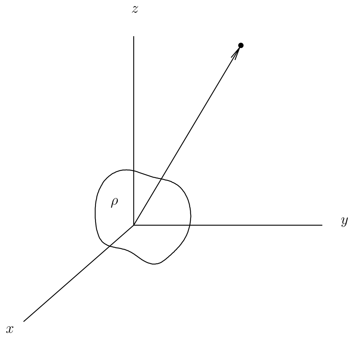
Figure 1:The origin of coordinates is placed inside a region to which a charge distribution and current distribution are confined. The field point is outside the charge and current distributions.
The quantities , , and that appear in the multipole expansions are moments of the charge and current distributions,
The dipole moment vector is the charge-weighted position vector, and the quadrupole moment tensor is the charge-weighted tensor . The tensors and are symmetric and traceless, and thus contain five independent components. These moments characterize the source distribution but are independent of position.
The nomenclature of the multipoles is explained in Table 1. Each pole is associated with an integer , and the name contains a Latin or Greek prefix indicating the number . We shall refer to them in general as -poles.
Table 1:The names of the multipoles are obtained by using Latin or Greek prefixes indicating a power of 2.
Pole | Numbers | |
|---|---|---|
Monopole | ||
Dipole | ||
Quadrupole | ||
Octupole |
About Nuclei and Nuclear Multipole Moments
We denote the spin of the nucleus by , reserving the symbol for the electron spin. We let the quantum number of the operator be , so that has eigenvalues . We denote the nuclear Hilbert space by , a -dimensional space in which the standard basis is . The nuclear Hilbert space consists of a single irreducible subspace under rotations. In actual stable nuclei, the spin ranges from to . For example, the proton, the nucleus of ordinary hydrogen, has , while the deuteron, the heavier isotope of hydrogen, has . The isotope used in atomic clocks has .
Not all the multipole fields that occur classically are allowed in the case of a nuclei. There are two rules governing the allowed multipole moments of the nucleus. The first is that electric multipoles of odd and magnetic multipoles of even are forbidden. To see why, consider what would happen if the nucleus had an electric dipole moment. Then the dipole term in (1) would be a (presumably small) correction to the potential seen by the atomic electron. Since the potential seen by the electron is , the perturbing Hamiltonian would be
The dipole moment vector is not a -number as in classical electrostatics, rather it is a (vector) operator acting on the nuclear Hilbert space, just like the magnetic moment . And just like , must be proportional to the spin, say, , because all vector operators on a single irreducible subspace are proportional. See Prob. Paragraph(a). Thus,
Now under parity the angular momentum is invariant, but the electron position vector changes sign. And under time reversal the angular momentum vector changes sign and does not. Thus we find that violates both parity and time reversal,
A similar argument applies to the other forbidden terms.
The presence of such terms would indicate a violation of both parity and time reversal. The weak interactions do violate parity, and we do know that time reversal (more precisely, CP) is violated at a very small level in certain decay processes (see 21. Parity{} and \timerev), so it is possible that the terms forbidden by this rule actually exist at a small level. For example, the neutron or the electron may have an electric dipole moment, but if such moments exist, they are certainly very small. There is currently considerable experimental interest in lowering the known upper bounds on these “forbidden” moments, or possibly even discovering a nonzero value for some of them, because a numerical value for one of these moments would shed light on physics beyond the standard model.
The experimentally known limits on the electric dipole moment of the neutron give rise to what is known as the “strong CP-problem” in particle physics. Theories of the strong interactions suggest that they should violate CP symmetry at a level that would show up as an electric dipole moment of the neutron that is larger than the experimentally known upper bound. Recall that the CPT theorem says that the product CPT is an exact symmetry of all quantum fields, so CP violation implies violation of time reversal. This suggests that there is some mechanism to suppress CP violation. One possibility that has been explored involves postulating the existence of a particle of very small mass, the “axion.” Nowadays the axion, in addition to solving the strong CP-problem, is looked upon as a candidate for dark matter, and extensive searches are underway to find it. Its discovery would be a major advance in both particle physics and astrophysics.
The second rule states that a -pole can occur only if . For example, the proton with can (and does) possess an electric monopole moment and a magnetic dipole moment, but not an electric quadrupole moment. The deuteron with can (and does) possess an electric quadrupole moment, but the alpha particle with can possess only the electric monopole moment. There are no hyperfine effects in , or with any other isotope with spin~0 (such as or ).
Lying behind this rule is the fact that the operator representing the -pole on the nuclear Hilbert space is, in fact, an order irreducible tensor operator. We have already studied the examples of the magnetic dipole moment and the electric quadrupole moment, which are respectively and irreducible tensor operators. In fact, the expansion of classical electric and magnetic fields into multipoles is an example of the decomposition of a space of fields on three-dimensional space into irreducible subspaces under rotations, each of which has an angular momentum value ( for monopole, for dipole, etc). The fields in question are classical fields, not quantum wave functions, but the transformation properties under rotations is exactly as presented in 13. Representations of the Angular Momentum Operators and Rotations\ and \orbamsph.
But the maximum order of an irreducible tensor operator on the nuclear Hilbert space with spin is . To see this notice that any operator that acts on the nuclear Hilbert space can be expanded as a linear combination of the operators , where (we suppress the index , which is constant):
where
Thus, the operators form a basis in the space of operators acting on the nuclear Hilbert space. But since the kets transform under rotations according to the irreducible representation , and since the bras also transform according to the same irreducible representation, the operator transforms according to
Each in the range occurs precisely once in this list, so on the nuclear Hilbert space there is precisely one scalar operator (to within a multiplicative constant), one vector, etc, all the way up to one order irreducible tensor operator. Equivalently, any operator that acts on the nuclear Hilbert space can be represented as a sum of irreducible tensor operators of order not exceeding . Operators with do not occur. See Prob. Paragraph(a).
To understand how the moments that are forbidden in the case of a nucleus or an elementary particle can occur classically, see the discussion in Secs. Energy Eigenstates in Isolated Systems and The Nucleus and the M"ossbauer Effect (it has to do with the fact that in the case of the nucleus, we are dealing with a single irreducible subspace under rotations).
Magnetic Dipole Hyperfine Effects. The Physical Picture
The only hyperfine effect we shall examine in these notes is the one due to the magnetic dipole moment of the nucleus. It turns out that if the electric quadrupole moment exists, then its effects are of the same order of magnitude as those of the magnetic dipole, so any realistic treatment requires that the two be treated together (unless selection rules make the quadrupole term vanish). In the following we will treat magnetic dipole effects in a single electron atom with nuclear spin , but to be realistic should not exceed . This condition holds in ordinary hydrogen with the proton as its nucleus, and at a certain point in the calculation we will specialize to that case.
A classical model of the effect will be useful in understanding what we do. To be specific we think of hydrogen. The proton at the center of the atom produces a magnetic dipole field in addition to the electrostatic, Coulomb field. The Coulomb field is rotationally invariant, but the magnetic dipole field depends on the orientation of the proton. As the electron moves in its orbit, which is largely determined by the electrostatic force, it also feels a force due to the proton’s magnetic field, which modifies the orbit somewhat. At the same time the electron’s spin has an energy of orientation in the proton’s magnetic field, and precesses in response. Also, the proton itself feels a magnetic field produced by the electron, both by its orbital motion and by its own magnetic moment, and precesses in response. Thus the orientation of the proton is not constant, but evolves in time as the electron executes its orbit. This picture makes it clear that the dynamics of the proton spin are coupled to the dynamics of the atomic electron, and that they must be handled together.
In the following we shall make a quantum mechanical analysis of these effects. Perhaps surprisingly, it turns out to be possible to obtain a closed formula for the shifts in the atomic energy levels, in terms of the expectation value of . In the case of hydrogen, the latter can be evaluated explicitly.
About Magnetic Dipoles
We begin by considering magnetic dipole fields in classical magnetostatics. A point magnetic dipole of moment situated at the origin of the coordinates produces a magnetic field , where
The vector potential falls off as and the magnetic field as at large , both with a nontrivial angular dependence. Both fields have a singularity at the origin that must be treated with some care in the quantum mechanical analysis of hyperfine effects.
We will do this by smearing out the point dipole moment over a sphere of small radius , producing a model in which the dipole is replaced by a uniformly magnetized sphere at the origin. Recall that in magnetostatics the magnetization is the dipole moment per unit volume, so we require
where is the constant magnetization inside the sphere and where is the volume of the sphere,
This model produces fields that are well behaved everywhere in space. When we are done with the quantum mechanical calculation, we will take in such a way that is constant, and we will find physical results that are finite and well behaved. Notice that in this limit, .
The problem of the uniformly magnetized sphere is a standard one in courses on electromagnetism. The vector potential at a field point can be computed as an integral over the source distribution inside the volume of the sphere,
The field point can be either inside or outside the sphere. The quantity in the square brackets is easily evaluated with some reasoning from electrostatics. The integral is the electrostatic potential produced at field point due to a uniformly charged sphere of radius and charge density . Thus, the negative gradient of that integral is the electric field produced by the same charge density. But by Gauss’s law, that electric field is times the amount of charge inside radius . Thus we have
Combining this with (12)--(14), we obtain
The exterior solution is identical to that of a point dipole, (11); in the region , one cannot tell from the field alone whether it is produced by a point dipole or a uniformly magnetized sphere of the same strength.
By taking the curl we compute the magnetic field,
where is defined in (2). The notation means the vector whose -th component is . Notice that is a symmetric and traceless tensor, something that becomes a irreducible tensor operator when reinterpreted as a quantum operator. The vector potential (16) is continuous at the radius ; the magnetic field (17), however, has a discontinuity there, due to a surface current.
To express both and in single formulas, we introduce the following functions:
and
Then we can write
and
where is the identity tensor.
When we take the limit , becomes a function that is concentrated inside a small volume with a value that goes to in such a way that the integral of over all space is the constant . This is the behavior of a function whose limit is a delta function, so we can write
As for , it has the limit,
The Hamiltonian and the Hilbert Space
We turn now to the atom in which the nucleus resides. In these notes we will be mainly interested in hyperfine effects in hydrogen and alkali atoms, the latter treated as atoms with a single electron (the valence electron) moving in a screened Coulomb potential.
In the following we use atomic units and take for the -factor of the electron, so . The Hamiltonian for the atomic electron is
where is the central force potential. This could be the Hamiltonian for the Zeeman effect, except that in this case the fields and are not external fields, rather they are the magnetic dipole fields of the nucleus. Thus, they are given by (20) and (21). We include in the Hamiltonian the fine structure terms , the sum of the three terms shown in (25), and terms responsible for the Lamb shift, since we wish to make a realistic treatment of hyperfine effects which are smaller than those just listed. We will not need to know much about the Lamb shift in the following analysis, except that it splits the energy levels in hydrogen to give them a dependence on .
The expressions (20) and (21) for and are the fields of a classical magnetic dipole at the origin, but now for use in the Hamiltonian (24) we must reinterpret as an operator acting on the nuclear Hilbert space, given in terms of the nuclear spin by
where is the -factor of the nucleus and is the nuclear magnetic moment (see \spinmagf.8). Thus, the Hamiltonian (24) must be interpreted as an operator acting the total Hilbert space
where , the electronic Hilbert space, is the product of its orbital and spin parts,
Basis states in can be defined as products of basis states in and in . For the obvious basis is the eigenbasis of , in the notation of 25. Fine Structure in Hydrogen and Alkali Atoms, which have energies . In alkalis the energies depend strongly on , and in hydrogen they depend on because of the Lamb shift. The obvious basis in is . Thus we define the basis states in ,
where we suppress the index in the shorthand notation on the right hand side, since it is a constant. We will call this the “uncoupled basis,” because the electronic angular momentum and nuclear angular momentum are not coupled. Of course, orbital and spin angular momentum have already been coupled to produce , so the basis (28) is really only partially uncoupled. These uncoupled basis states are eigenstates of on the whole Hilbert space . The energy does not depend on the quantum numbers or , so the energy eigenstates are -fold degenerate.
Now we expand the kinetic energy in the Hamiltonian (24) as in 26. The Zeeman Effect in Hydrogen and Alkali Atoms\ and neglect the term in , writing the result as , where
and
Here we have used the fact that our is in Coulomb gauge, , so . We write the two terms in as and . For we use and (25) and (20), rearranging the triple product,
This gives
where we have set
for the product of the effective magnetic moments of the electron and the nucleus (including -factors). As for , we rearrange it similarly, obtaining
Notice that is a kind of spin-orbit interaction (but it is the spin of the nucleus, not the spin of the electron), and is a kind of spin-spin interaction.
Properly we should only take the limit after we have formed matrix elements, but in many books this limit is taken before, resulting in the formulas,
and
The terms involving are called “Fermi contact terms,” because they vanish except when the electron and nucleus are in contact with one another (, and in honor of Fermi, who first carried out the calculation presented in this set of notes.
The Perturbation Calculation
Both terms (32) and (34) in the perturbing Hamiltonian have the form of dotted into a vector that is constructed out of electronic operators, that is, operators that act only on the electronic Hilbert space. Since the angular momentum generates rotations that rotate electronic vectors, while generates rotations that rotate itself, the dot products in are not invariant under either electronic rotations alone or under nuclear rotations alone. For this reason, does not commute with either or , and the uncoupled basis (28) is not the best one for carrying out the perturbation calculation (see \finestruc.5).
The dot products in question, however, are invariant under total rotations of the system, electronic plus nuclear, which are generated by the total angular momentum of the system defined by
This suggests that we couple together and to create eigenstates of and . We will call the result the “coupled basis”; it is given by
where the final scalar products are the Clebsch-Gordan coefficients.
In the coupled basis the matrix elements we need to consider for degenerate perturbation theory are
where the unprimed indices on the two sides specify the degenerate unperturbed energy level , while the remaining indices specify the basis inside the degenerate eigenspace of the unperturbed system. But since , and since if commutes with it commutes with any function of such as , the matrix (39) is diagonal in both and , and the primes can be dropped. We need only compute the diagonal matrix elements to find the energy shifts, and once again we have succeeded in doing a degenerate perturbation calculation without diagonalizing any matrices. Thus we have
We now evaluate these matrix elements for the case . In this case the contact terms do not contribute in the limit , because the wave functions go as near , and thus vanish at when . As for the other terms, we take the limit so , and write the result in the form
where
where we use (2). Note that is a purely electronic vector operator.
We simplify (41) by using the projection theorem (see The Projection Theorem and Prob. Paragraph), which tells us that an operator such as , which is a vector under rotations generated by , sandwiched between eigenstates of with the same value on both sides, can be replaced by an operator proportional to :
Thus
Now the two dot products can be simplified. First, by (37), we have
Next, we use (since ) to write
where a term has cancelled. Then, since and since , the final term in (46) simplifies,
which cancels . The result is simply
Then, with (45) and (48), the energy shift (44) becomes
where the final expectation value of can be reduced to a purely spatial matrix element with respect to the state exactly as in \finestruc.7. Specializing to hydrogen and using (33) and (53), we find
where we have introduced a factor of ( is the Bohr radius) to make the answer have dimensions of energy (thus it is now valid in ordinary units).
(50) is the final expression for the hyperfine structure energy shift in hydrogen in the case . However, one can show that the same answer holds also in the case , so (50) applies in all cases.
The New Energy Levels
The energy levels were before the hyperfine interactions were turned on, but since in (50) depends on , they now have the form . The energy eigenstates are , and are -fold degenerate, since the energy does not depend on . This is precisely the situation expected of a generic system invariant under rotations; the energy eigenspaces consist of a single irreducible subspace under rotations (see Secs. Energy Eigenstates in Isolated Systems--The Nucleus and the M"ossbauer Effect); and the degeneracy present is explained by rotational invariance alone.
The energy shift (50) causes the fine structure levels in the Dirac picture of hydrogen to split, giving rise to hyperfine multiplets. For example, the ground state splits into two levels and , of which is lower since by (50) the energies are an increasing function of . This level is the true ground state of hydrogen. It is nondegenerate. The level is 3-fold degenerate, and lies above the ground state by an energy of approximately 1.42~GHz in frequency units, or 21~cm in wave length units, or 0.068~K in temperature units. Since for these states, the total angular momentum is really just the total spin , and the and states are the spin singlet and triplet states, respectively. The electron and proton spins are antiparallel in the ground (singlet) state; when one of the spins is flipped to make them parallel (the triplet state), the energy is raised.
Similarly, other states including the and states split into an and pair. The state in the Dirac picture splits into an and pair.
Electric dipole transitions between the various hyperfine levels are governed by the matrix element,
The selection rules for this matrix element follow from the Wigner-Eckart theorem and parity. The Wigner-Eckart theorem can be used three times, once for each of the three angular momenta , and , since is a irreducible tensor operator with respect to rotations generated by any of these angular momenta. Thus, the matrix element (51) vanishes unless the following selection rules are satisfied:
The exclusion of comes from the fact that , so if , then the matrix element vanishes. The only reason we do not also exclude is that is half-integral, and cannot take on the value 0. And the only reason we do not make a special case of excluding is that that case is already excluded by parity.
The hyperfine splitting of the level in hydrogen is particularly interesting. The separation between the and hyperfine levels is 1.42~GHz, or 21~cm in wavelength units. Electric dipole transitions between these two levels are forbidden by parity, but magnetic dipole transitions are allowed. (One can see this from another standpoint: since spins do not interact with electric fields, an electric dipole transition cannot flip the spins to convert the triplet to the singlet state. But magnetic dipole transitions can.)
The 21~cm line is quite important in radio astronomy. Spiral galaxies typically possess large clouds of atomic hydrogen, which radiate at the 21~cm wavelength. A population of the excited state is maintained by collisions; the temperatures prevalent in the clouds are high enough that the populations of the ground state and the first excited state are determined mostly by the degeneracies (1 for and 3 for , although there is some effect due to the Boltzmann factor). By measuring Doppler shifts, the state of motion of the clouds can be measured. In this way, it was first proven that the Milky Way is a spiral galaxy. The 21~cm line is also important in absorption spectra, which can be used to determine the temperature of the clouds of atomic hydrogen.
Molecular hydrogen has a completely different hyperfine structure from atomic hydrogen, arising from the spin-spin interaction of the two protons in the molecule. The transitions between the hyperfine levels of molecular hydrogen are in the megahertz range of frequencies.
Problems
Problem 1.
A problem on the hyperfine interaction in hydrogen.
(a) (50) was derived in the case . Show that it also applies in the case . Hint: Use the fact that the components of the tensor , defined in (2), are times linear combinations of the , for . This is related to the fact that is the Cartesian version of an order 2 irreducible tensor.
(b) Our analysis of the hyperfine interaction in hydrogen has included the energy of interaction of the electron with the magnetic dipole field produced by the proton, but it seems that we have not included the energy of interaction of the proton spin with the magnetic field produced by the electron. As seen by the proton, the electron produces a magnetic field for two reasons: first, it is a charge in motion, therefore a current, which makes a magnetic field. This is the magnetic field due to the orbital motion of the electron. Next, the electron has a magnetic moment of its own, which makes a dipole magnetic field. This is the magnetic field produced by the spin of the electron.
Work out an expression for the energy of interaction of the proton spin with the magnetic field produced by the orbital motion of the electron. Follow the analysis of the spin-orbit interaction in The Hamiltonian, but run it backwards. That is, putting primes on the fields in the electron rest frame and no primes on fields in the proton rest frame, use Coulomb’s law to write down the field of the electron in its own rest frame, then Lorentz transform to the lab frame to get (call this , the magnetic field due to the orbital motion of the electron). Then the energy of interaction of the proton with this magnetic field is , where is the proton magnetic moment. Notice that unlike the analysis of The Hamiltonian, there is no factor of from Thomas precession, because the proton frame is not accelerated.
Now use (21) in the limit to obtain the magnetic field produced by the dipole moment of the electron at the position of the proton. Call this , and write down an expression for the energy of interaction .
If you add these terms to the Hamiltonian ((29) plus (30)), does it change the energy shifts (50)? These energy shifts are confirmed experimentally (for example, by the 21~cm line). What is wrong?
(c) Compute the hyperfine splitting of the ground state of positronium in wavelength units. Notice that in positronium, the fine structure and hyperfine structure are of the same order of magnitude.
Now some remarks about part (c). The interesting thing about this calculation is that the answer based on what you now know is actually wrong, because it omits a virtual process (a Feynman diagram) in which the positron and electron annihilate into a photon, which then materialize back into a positron and electron.
The analysis of this process requires quantum field theory. The Hamiltonians we usually use in atomic, molecular and solid state physics, expressed in terms of a finite number of particles and a finite number of degrees of freedom, are only valid up to a certain degree of accuracy, beyond which interactions with the infinite degrees of freedom in various fields (electromagnetic, electron-positron, strong interactions, ) cannot be ignored. The first place where this occurs in hydrogen is with the Lamb shift. In positronium, it happens at the level of the fine structure (in positronium, the hyperfine structure is considered part of the fine structure).
Problem 2.
In our derivation of the energy shifts (\eqr\cn.50), we assumed that hyperfine effects were much smaller than the Lamb shift. This is what allowed us to assume that the values on the two sides of the matrix element (\eqr\cn.39) were the same. Compute the hyperfine energy shifts for the and levels in hydrogen, and compare to the Lamb shift. Make a sketch of the energy levels like that in Fig.~\figr\finestruc.3, including the hyperfine structure (but you can omit the levels). It’s convenient to measure energies in GHz.
Problem 3.
Hyperfine transitions in alkali atoms, usually cesium or rubidium, are used in atomic clocks. Atomic clocks can also be based on hydrogen. Hydrogen and alkali atoms have one unpaired electron, so . When this is coupled to the nuclear spin , where , the resulting total angular momentum is . Thus, there are two hyperfine levels, characterized by their values. For example, in cesium, where , we have either or .
In the usual atomic clock an atomic beam is passed through a region of space with an oscillating magnetic field produced by an RF oscillator, much as in the magnetic resonance experiments discussed in 14. Spins in Magnetic Fields. When the frequency of the oscillator is close enough to the hyperfine transition frequency, it causes the hyperfine state to change, thereby modifying the trajectory of the atom in a subsequent Stern-Gerlach apparatus. A feedback mechanism locks the frequency of the oscillator onto the hyperfine transition frequency, so that only atoms following a certain trajectory, corresponding to a certain } value, are passed. See R.~E.~Beehler, R.~C.~Mockler and J.~M.~Richardson, Metrologia 1, 114(1965).
Hyperfine transition frequencies in the alkali atoms and hydrogen are among the most accurately known physical quantities. In fact, as mentioned, the second is currently defined in terms of the hyperfine transition frequency in cesium. As for hydrogen, measurements of the transition frequency give [see L.~Essen, R.~W.~Donaldson, M.~J.~Bangham and E.~G.~Hope, Nature (London) 229, 110(1971)].
Unfortunately, to flip the hyperfine state we need a background field , in addition to the oscillating magnetic field, as explained in 14. Spins in Magnetic Fields, and this modifies the hyperfine transition frequency. Thus, it is necessary to know how the hyperfine transition frequency depends on the background field in order to make the correction. Also, the accuracy of the clock now depends on the accuracy with which we can measure .
In this problem for simplicity we will work with hydrogen, but the theory is not much more complicated for atoms such as cesium.
(a) Let be the energy difference between the two hyperfine states in hydrogen (the and states). This can be calculated from (50), or from the experimental value of . (They should agree, and since you shouldn’t believe everything you read you might want to check that they do.) To estimate the magnetic field strengths we will be talking about, let us note that the energy of interaction of an electon spin with a magnetic field is of the order of , and let us define a field strength by
where is the Bohr magneton. Evaluate in Gauss or Tesla (see Magnetic Moments). This is roughly the field strength at which the effect of an external field is comparable to the hyperfine interaction. When the hyperfine structure seen at is strongly modified by the external field. We will want to operate the atomic clock at field strengths , so that the corrections due to are small.
(b) Write the Hamiltonian for the hydrogen atom as where
Here is the Hamiltonian in the electrostatic model, are the fine structure corrections studied in 25. Fine Structure in Hydrogen and Alkali Atoms, are terms responsible for the Lamb shift, are the hyperfine corrections, what was called in (30) (which is presented in atomic units), and contains terms representing the interaction of the atom with the external field . By treating both and as of the same order of magnitude, we will be able to see what happens to the hyperfine structure as the external field is varied from zero up to the value and beyond.
The answers to this problem do not depend on and it can be ignored for the purpose of doing the problem. We include it anyway in (57) because it is really there. It is worthwhile thinking about why it does not affect the answers.
Write out an expression for , including the interaction of the proton spin with the magnetic field . The latter interaction is small but it has a qualitative effect on the energy level diagram so we will keep it. Neglect other terms that are very small. Express as a multiple of , and use the abbreviation,
I suggest you use the gauge , so that and .
(c) Find the energy shifts of the ground state () of the hydrogen atom in the model represented by due to .
I suggest you write and for the energies of the hyperfine states and , respectively, relative to the energy of the level in the model represented by . These are the energies computed from (50) with and . Note that
Sketch the behavior of the energy levels as a function of , as is varied from zero up to and beyond.
(d) You will see that when the effect of is to split the energy levels indicated by (50) in proportion to their values, with an effective -factor, as in the weak field Zeeman effect studied in 26. The Zeeman Effect in Hydrogen and Alkali Atoms. Therefore when we operate the atomic clock, we have to decide which pair of magnetic substates we will use for the transition. Actual atomic clocks use the two substates (for example, in cesium it is the transition between and ). Explain why this is the best choice.
(e) Let be the hyperfine transition frequency in hydrogen in the absence of a background field , as quoted above, let be the frequency of the transition when there is a background field , and let . When , express as a function of the dimensionless ratio .
Suppose , which is known to within an accuracy of . Find the corresponding accuracy . This is the limitation on the precision with which the clock can measure time, due to the accuracy in the measurement of .