38. The Lippmann-Schwinger Equation and Formal Scattering Theory
Introduction
In earlier lectures we studied the scattering of spinless particles by central force potentials. Such problems are tractable because the Schr"odinger equation is separable in spherical coordinates, and we were able to reduce everything we wanted to know to the properties of radial wave functions. But those are a rather restricted class of problems.
In these notes we apply Green’s functions and Green’s operators to scattering problems. Although we mainly treat potential scattering in three dimensions, in fact the techniques we develop have a much broader applicability. We shall see that Green’s functions lead to powerful operator methods for treating scattering problems that allow us to derive both exact results and approximation methods in scattering theory. These can be generalized in a variety of ways, for example, to relativistic and field theoretic problems.
We begin by deriving the Lippmann-Schwinger equation, a formulation of the scattering problem in terms of an integral equation that is central to all further developments. An asymptotic analysis of this equation leads to an exact relation between the scattering amplitude and the properties of the wave field at small radii (where the potential is active). This is ultimately the basis of several exact results involving the scattering amplitude. The Lippmann-Schwinger equation also easily leads to a simple approximation scheme, the Born series, as well as to an intuitive and quantitative criterion for the conditions of validity of the Born approximation. Then we develop some of the properties of the exact Green’s operator for the system, and show how all results of interest in scattering theory can be expressed in terms of it. Then we discuss the transition operator, in terms of which the exact scattering amplitude can be expressed, which allows a neat determination of the effects of various symmetries (parity, time reversal, etc) on the scattering amplitude. Finally we discuss the orthonormality relations satisfied by the scattering states.
This material is background on the -matrix, which we will not discuss in these notes, but which is a central object of investigation in advanced treatments of scattering theory, especially in relativistic quantum mechanics.
The Lippmann-Schwinger Equation
We consider potential scattering of a spinless particle in three dimensions. We write the Schr"odinger equation in the form (12),
where since we are interested in scattering solutions. The potential is not necessarily rotationally invariant, but we do assume it falls off sufficiently rapidly as . We will be more quantitative about this condition below. We treat the right-hand side of (1) as a driving or source term, so the general solution can be written
where is a solution of the homogeneous equation, that is, , and is an energy-dependent Green’s function for the free-particle Hamiltonian . (As in 37. Green’s Functions in Quantum Mechanics, the 0-subscript means “free particle.”) The homogeneous solution is a free-particle wave function of energy . With different choices for and , we get different solutions of (1).
Because we are interested physically in scattered waves that are radiated outward from the scatterer, we take to be the outgoing free-particle Green’s function, , given by (100). We will examine the boundary conditions on the scattered wave more carefully in a moment. As for the homogeneous solution , we take it to be a plane wave with wave vector ,
and we interpret it as the incident wave. We just write for the plane wave of wave vector in ket language. As discussed earlier, the scattered wave is the difference between the exact solution and the incident wave, a free particle solution. Our plane waves are normalized so that
With this choice of Green’s function and incident wave, (2) becomes
This is the Lippmann-Schwinger equation. It is not so much a solution of the original Schr"odinger equation (1) as a reformulation of it in terms of an integral equation, since the unknown wave field occurs both on the left-hand side and under the integral on the right-hand side.
The Lippmann-Schwinger equation (5) contains both an energy eigenvalue and a wave vector . These are related by the
in spite of the fact that is not a solution of the exact Schr"odinger equation (at least not where ). This is because is a solution of the homogeneous equation , whose energy parameter is the same as the energy eigenvalue of the exact Schr"odinger equation (1). More physically, the experimenter is free to launch particles at the target with any value of momentum, but the energy and momentum are related by the free particle relation since the particles are free where they are launched, in the asymptotic region. Moreover, the energy of the particles in the beam is the same as the energy eigenvalue of the corresponding solution of the Schr"odinger equation. This is plausible physically because a uniform beam of particles directed against a target produces after a while a steady state, statistically speaking, in which a definite number of particles per unit time are scattered into any given element of solid angle. It is plausible that this steady state should correspond to a solution of the Schr"odinger equation with energy , since measuring the energy of the particles in the asymptotic region produces the value .
This physical picture suggests (correctly, as it turns out) that the Lippmann-Schwinger equation has a unique solution for a given wave vector (which determines ). That is, for a given , there is a unique solution satisfying the given boundary conditions (which consist of the given incident wave of wave vector , plus the fact that the scattered waves are purely outgoing). This is in contrast to the original Schr"odinger equation, the differential equation (1), which has many solutions for a given energy . This is clear physically, since the experimenter is free to direct the beam against the target from any incident direction, thereby generating different states of the same energy. We will write to emphasize the -dependence of the solution. With this slight change of notation, the Lippmann-Schwinger equation becomes
or, in ket form,
where it is understood that and are related by the free-particle relation (6). As usual, the ket form has the advantages of compactness and generality. Finally, substituting the form of the free particle outgoing Green’s function (100) into (7), we have the explicit integral equation,
The Lippmann-Schwinger equation is a fundamental result, as important for scattering theory as the Schr"odinger equation is for the rest of quantum mechanics. As we shall see, it opens the door to many exact results in scattering theory as well as various approximation methods.
There are obviously many variations on this derivation. For example, the incident wave need not be a plane wave. For another example, the unperturbed Hamiltonian might include part of the potential, presumably a part such that can be solved, while contains the rest of the potential. For example, in proton-proton scattering we might take to include the (long-ranged) Coulomb potential of the two protons, while would contain the short-ranged nuclear potential. In this case, would be a Coulomb solution of positive energy.
The Scattering Amplitude
The Lippmann-Schwinger equation in the form (9) represents the scattered wave as a superposition of outgoing spherical waves, radiating from each point of space where . The integration over in (9) represents this superposition. In general, the different spherical waves are not in phase with one another, and their interference gives rise to the angular dependence of the scattered wave.
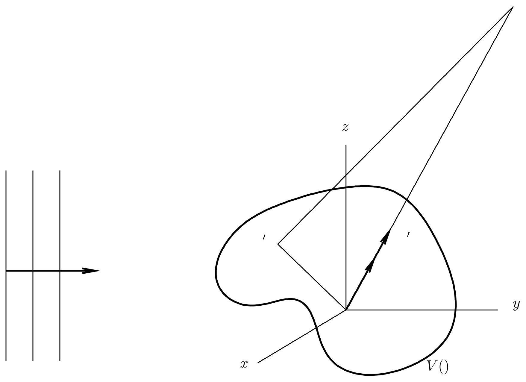
Figure 1:An incident plane wave with wave vector is launched against a localized potential. Observation point is in the asymptotic region, while is a variable of integration that runs over the region where . Wave vector has the same magnitude as the incident wave vector , but points in the direction of the observation point.
Let us assume for the moment that the potential rigorously vanishes outside some radius , and let us consider the case in which in (9) is well outside this radius, . We interpret as an “observation point” (see Figure 1). Then the variable of integration in (9) is limited by , and we have over the entire range of integration. Therefore we may expand the integrand in powers of . We are only interested in the dominant term as , but different parts of the integrand must be expanded to different orders in . For example, in the exponent we have
where is a unit vector from the scatterer to the distant observation point. Now we define a scattered wave vector,
which has the same magnitude as the incident wave vector (because the scattering is elastic), and which also points from the scatterer to the observer. Then
The first term is large as , while the next term is independent of . We stop at this order of the expansion, because the following term is down by a factor of , so it goes to zero as . As for the denominator in (9), we expand it to lowest order,
since the next term goes to zero faster than as .
Altogether, when is in the asymptotic region the Lippmann-Schwinger becomes
dropping correction terms that go to zero faster than as . The integral is now independent of the magnitude of , but depends on its direction through . The scattered wave has the form of times a function of the scattering angle, that is, the asymptotic wave field can be written as
where is the scattering amplitude. We previously argued on somewhat intuitive grounds that the asymptotic form of the wave field must have this form, and we proved that it does so in the case of central force scattering. Now we have proved it for scattering from a potential of any shape.
We assumed above that the potential rigorously vanishes outside some radius. If this is not true, it can still be shown that the asymptotic form (14) is correct, as long as the potential goes to zero faster than as . As a practical matter, this covers all potentials of interest except the Coulomb potential.
We have previously written the scattering amplitude as , referring to the spherical coordinates of some coordinate system, but now we are writing it in the coordinate-independent form , specifying both the incident and scattered vectors. The notation is slightly misleading, since is not an independent function of both vectors, whose magnitudes are required to be equal. By comparing (14) and (15), we can read off an expression for the scattering amplitude,
where we use (4). This is an exact expression for the scattering amplitude, a property of the wave field in the asymptotic region, in terms of an integral involving the wave field in the region where the potential is nonzero. Thus it provides a connection between the region at large radii and the region at small radii. (16) cannot be used immediately to calculate the scattering amplitude unless we know the values of the exact solution at small radii, but it is important for deriving general relations concerning the scattering amplitude as well as for developing approximation methods.
The Incoming Solutions
What would have happened if we had used the incoming Green’s function in the integral equation (2)? The solution would still be unique for given wave vector of the wave , but it would not be the same solution we have been discussing. Instead, it would consist of waves streaming inward from infinity toward the scatterer, which would combine with plane wave to form an exact solution of the Schr"odinger equation with energy . These solutions would obviously be impossible to set up experimentally, but they are perfectly good solutions of the Schr"odinger equation from a mathematical standpoint, and, as it turns out, they are also useful in scattering theory. When it is necessary to distinguish the two types of solutions, we will write them , where the sign indicates the type of Green’s function used (, ). If we omit the sign, the outgoing solution will be assumed. These two types of solutions satisfy the Lippmann-Schwinger equations,
or, in ket language,
An Integral Equation for Bound States
It is also possible to formulate an integral equation for the bound states. When , there can be no homogeneous solution as in (2), because no free particle solution for has the right behavior at infinity. Therefore there is only the inhomogeneous term. Furthermore, both Green’s functions are equal for , as shown in (100), and indeed, there is only one Green’s function with the right behavior at infinity. Thus we obtain the following integral equation for the bound states:
which can be satisfied only for discrete values of .
The Born Series
Let us write the Lippmann-Schwinger equation (8) in the form
which makes it clear that if we could invert the operator on the right-hand side, we could solve explicitly for the solution . (We henceforth drop the hat on the Green’s operator, it being fairly clear when an operator is being referred to and when a function.) We denote the required inverse by
where is called the M\o ller scattering operator. It is an operator that (for the given energy ) maps the incident plane wave into the associated, exact scattering solution ,
Similarly, we define an incoming version of this operator,
which is useful for finding incoming solutions,
More generally, we can define an operator , depending on a complexified energy,
so that
(This is not quite standard notation. Most references on scattering theory define a M\o ller wave operator, call it , that is independent of energy. The two operators have the same effect when acting on plane waves, however: , where is related to by the free particle relation.)
A simple approach to obtaining a useful expression for is to treat as small and expand the inverse operator in a power series. This gives
or, by (26),
When this series is applied to the Lippmann-Schwinger equation in the form (20), it gives
This is called the Born series for the scattering solution . When it is truncated at -th order in the potential , we speak of the -th Born approximation. Similarly, the expansion (28) can be substituted into the expression (16) for the scattering amplitude, yielding
which is the Born series for the scattering amplitude. Again, if we truncate at -th order, we obtain the -th Born approximation to the scattering amplitude.
The Born series can also be obtained by a method of successive approximations. If we take the Lippmann-Schwinger equation in the form (8) and substitute the left-hand side into the right-hand side, we obtain
an exact equation in which the unknown wave function has been pushed into a second order term in . By substituting (8) into (31) again, the term containing can be pushed to third order, etc. This procedure also generates the terms of the Born series, but with an explicit remainder term.
We shall examine the conditions of validity of the Born approximation in a moment, but for now we just remark that the series does not necessarily converge, and the Born expansion is only useful in some problems. Obviously it will work best when is small in some sense.
The first Born approximation to the scattering amplitude is
where is the Fourier transform of the potential using the convention (83), and where (times ) is the momentum transfer in the scattering. On taking the square of the scattering amplitude, we obtain the cross in the first Born approximation,
which agrees with our earlier result (86) from time-dependent perturbation theory. Although the scattering amplitude in the first Born approximation only depends on the difference between the incident and scattered momenta, this is not true in higher Born approximations, as one may easily see.
The first Born approximation gives the same result as first-order, time-dependent perturbation theory because there is a close relationship between the Dyson series (in the time domain) and the Born series (in the energy domain). Both are straightforward power series expansions in powers of the potential . The Born series, however, makes it easier to analyze the conditions of validity of the approximation, a subject to which we now turn.
Conditions of Validity of the Born Approximation
Let us write the Lippmann-Schwinger equation and the first Born approximation for the scattering solution side-by-side to compare them:
This shows that the scattered wave as computed by the first Born approximation is a good approximation to the exact scattered wave, everywhere in space, if the exact solution is approximately given by the incident wave at small radii where the potential is substantially nonzero. This leads to the intuitive conditions of validity of the first Born approximation: the approximation is good if the potential does not distort the incident plane wave too much in the neighborhood of the potential itself. This in turn shows that the Born approximation is good if the potential is weak or if the incident energy is high (since in that case the incident particles blast through the potential without being deflected very much).
To be more quantitative, we follow Gottfried, Quantum Mechanics and introduce the dimensionless quantity,
which we want to be small in the region where is largest. The quantity depends on , but we evaluate it at , for a (hopefully) typical point inside the scatterer. Then depends only on . Using the Lippmann-Schwinger equation and evaluating the integral transform at , we get
Since this is only an estimate, we replace with ,
dropping the primes on the dummy variable of integration. If is central force, then we can do the angular integration, obtaining
The quantity should satisfy if the Born approximation is a good one. Our argument leading to this criterion is not air-tight, but the criterion is useful nonetheless.
Consider, for example, the Yukawa potential,
where in comparison to (122) we have set so that is the effective range of the potential. Then the integral (38) can be done, yielding
This has the limits,
Small means that the incident wave length is much larger than the range of the potential; recall that in this case we have predominantly -wave scattering. In this case, the validity of the Born approximation is equivalent to the requirement that the Yukawa potential (if attractive) should be so weak that it does not support any bound states. Large means that the wavelength is small compared to the range of the potential. Notice that in the limit , which takes the Yukawa potential to the Coulomb potential. The conditions of validity of the Born approximation are not met for any for Coulomb scattering, as remarked earlier (see Example: The Yukawa Potential).
The Exact Green’s Function
So far in our applications of Green’s functions to scattering theory we have only used the unperturbed Green’s function, . But it turns out that many of the interesting quantities in scattering theory can be expressed in terms of the exact Green’s function or operator for the system. Let us recall the definitions of the resolvent operators,
which are well defined as long as is not equal to any eigenvalue of the corresponding Hamiltonian (either discrete or continuous). The Green’s operators for real energy are defined by setting and taking , when that limit exists (which it does as long as is not equal to any discrete, bound state eigenvalue). It was remarked in 37. Green’s Functions in Quantum Mechanics\ that the exact resolvent contains all the physical information we might be interested in about the given system, including the scattering solutions and amplitudes. We will now show how this comes about.
There are a number of useful relations connecting the exact resolvent and the unperturbed one that follow by just playing around with the definitions (42). For example, for any not on the real axis, where the inverses of and are defined and unique, we have
where the two versions differ by factoring out to the right or to the left. Now multiplying the first identity from the right and the second from the left by , we obtain
Finally, we multiply the first equation from the left and the second from the right by , to obtain
These are two identities connecting the exact and unperturbed resolvents in which only the order of the factors in the last term is different.
Equations~(46) can be regarded as Lippmann-Schwinger equations for the exact Green’s function. To see this, we first set and take to get the outgoing Green’s operators. Next we sandwich both equations between and to convert them into the language of Green’s functions instead of operators. Finally, we consider the unknown, exact Green’s function as being analogous to the unknown, exact wave function in the Lippmann-Schwinger equation, while the (known) unperturbed Green’s function is taken to be analogous to the incident plane wave . For example, this procedure applied to (46) gives
which should be compared to (7). In this case the effective Lippmann-Schwinger equation defines the dependence of on the field point . The analogous procedure applied to (46) gives a Lippmann-Schwinger equation that defines the dependence of on the source point .
Now we rearrange (46) as we did with (30),
which shows that
where is the M\o ller wave operator defined by (27). We see that knowledge of not only allows us to convert the incident plane wave into the exact scattering solution (see (22), but it also allows us to convert the unperturbed resolvent into the exact resolvent. (50) also makes it easy to expand the exact resolvent in a Born series, expressed in terms of the unperturbed resolvent,
Another interesting relation follows by solving (50) for and then using (45),
In other words, from the definition (25) of , we have
We see that the inverse of , needed to solve the Lippmann-Schwinger equation, can be expressed in terms of the exact resolvent. Thus the exact scattering solution can be written,
again showing how knowledge of the exact Green’s function allows us to determine exact scattering solutions.
The Transition Operator
Let us return to (16) for the scattering amplitude and substitute (54) into it. We write the result as
where , the transition operator, is defined by
(55) is a somewhat more symmetrical representation of the scattering amplitude than (16), because we have plane wave states on both sides of the matrix element. The transition operator incorporates all the complexities of the scattering process, and (55) is exact. Notice that if is replaced by the potential , we obtain the first Born approximation to the scattering amplitude. The transition operator is not Hermitian, but rather satisfies
where we use the fact that
The transition operator, or -operator for short, is useful for exploring the effects of symmetry on the scattering amplitude. This is an important question experimentally, when the fundamental symmetries that are obeyed or broken by some interaction are under investigation.
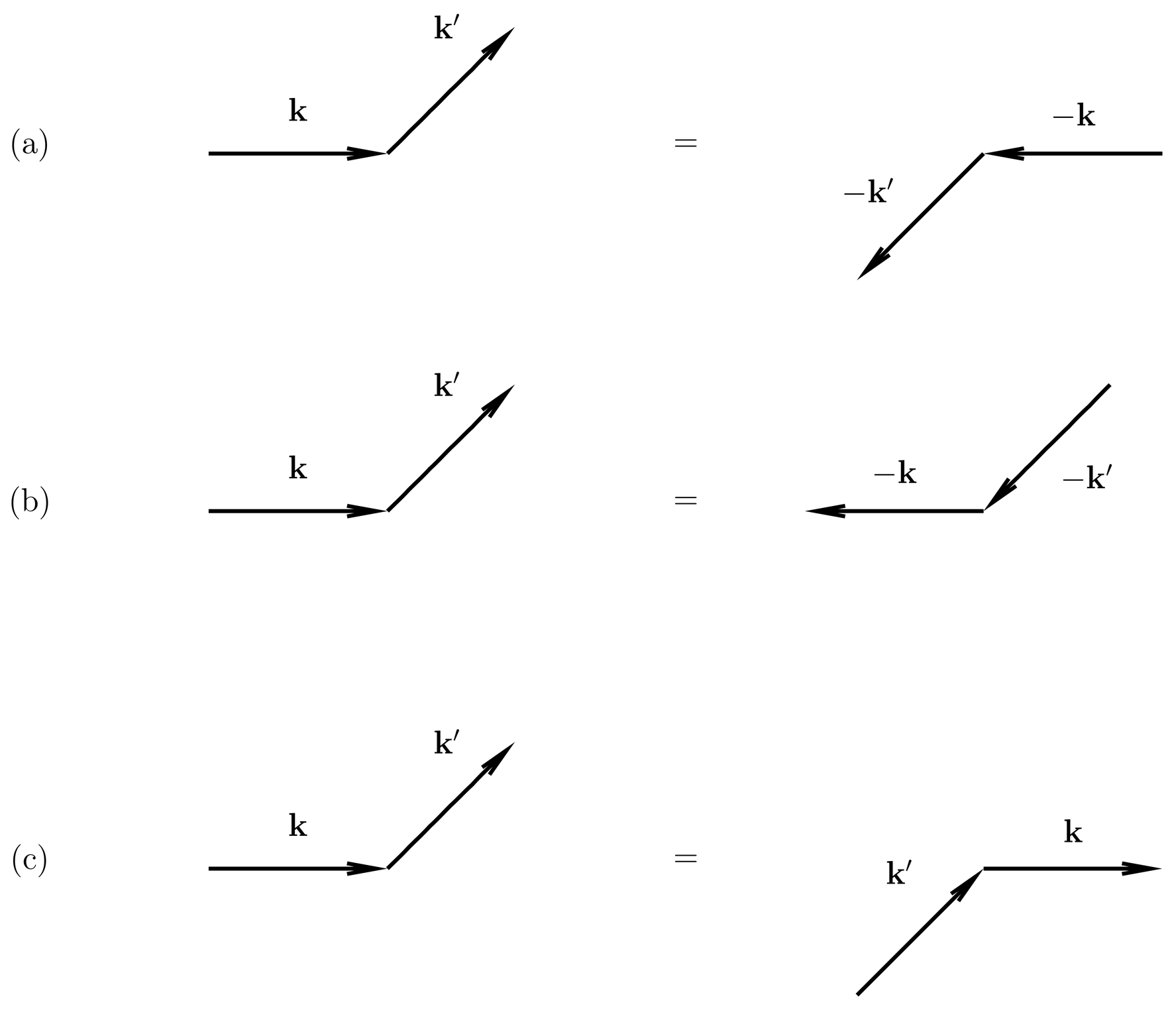
Figure 2:Effects of various symmetries on the scattering amplitude: (a), parity; (b), time-reversal; (c), parity and time-reversal.
We begin with parity (see 21. Parity). The action of parity on plane wave states is given by . Suppose that the Hamiltonian commutes with parity, so that and . Then commutes with any function of , so that
From this and (56) it follows that . Then we have
or,
This is illustrated as case (a) in Figure 2.
Next let us consider time-reversal (see 22. Time Reversal). The action of time-reversal on the (spinless) plane wave states is given by , since the wave function is transformed into its complex conjugate [see (51)]. Suppose that commutes with the Hamiltonian , and therefore with , . This does not mean that commutes with , for we have
since the antiunitary turns into . (More pictorially, we can say that reversing the direction of time turns the outgoing Green’s operator into the incoming Green’s operator.) Now (56), (57), and (62) imply
Now let us examine the effect of time-reversal invariance on the matrix elements of the -operator. We have
where the parentheses are used to indicate that the time-reversal operators act to the right, and where in the third equality we have reversed the direction in which is acting, and used (28). Thus, time reversal invariance implies that the scattering amplitude satisfies
This property is called microreversibility, and it is illustrated in case (b) in Fig.~lippschw-1.
Finally, if both parity and time-reversal are symmetries of the Hamiltonian, then we have
This property is called detailed balance, and it is illustrated in case (c) in Fig.~lippschw-1.
Orthonormality of the Scattering Solutions
We shall now derive the orthonormality relations for the exact scattering states . These relations are not easy to derive directly from the Schr"odinger equation or from the integral equation (7), but they can be easily obtained with the help of our various identities involving Green’s operators. We begin by using (54) to transform the scalar product of two exact scattering states,
where . The second term of this equation can be written,
where we have allowed to act to the left on , which brings out the eigenvalue . As for the first term on the right in (68), we first write down the Hermitian conjugate of the Lippmann-Schwinger equation (8), with and replaced by and ,
where we have used (58). Then we have
where we have allowed to act to the right on , which brings out the eigenvalue . Now combining (69) and (72), we obtain
a simple result.
Although the exact scattering states are orthonormal, they are not complete in general, because of bound states. All bound states of the Hamiltonian are orthogonal to all scattering states,
because they are eigenfunctions of the Hamiltonian with different (positive and negative) energies.
The completeness relation relation is
This can be proved by a contour integration that inverts the definition of the Green’s operators. We will not go into details here.
Problems
Problem 1.
This problem is a variation on Sakurai, {\it Modern Quantum Mechanics}, problem 7.1.
(a) Find the free-particle Green’s function in one dimension,
where
Do this for both and , as in the 3-dimensional case discussed in 37. Green’s Functions in Quantum Mechanics. Also find . Show explicitly that they satisfy
You may find it useful to note that
and
The Heaviside step function is defined by (20).
(b) Write down a 1-dimensional version of the Lippmann-Schwinger equation for an exact scattering solution associated with an incoming (from the left) free particle state . The exact solution satisfies the Schr"odinger equation in a potential , which you can consider to be localized. Consider asymptotic forms (large ) and find expressions for the transmission and reflection amplitudes and which are analogous to (32) in three dimensions. These amplitudes are defined by
(c) Consider the potential,
This potential can be seen as the limit of a rectangular barrier (for ) with width and height as . The attractive case is similar.
Solve the Lippmann-Schwinger equation directly, and write out explicit forms for the wave function for and . To help the reader, please use the abbreviation,
as much as possible. Note that is dimensionless. Compute and in terms of and show explicitly that .
(d) The operator equation,
was proved in lecture. It is a kind of Lippmann-Schwinger equation for the exact Green’s function. Write this out as an integral equation for the exact Green’s function, assume the potential is given by (83), and solve for . Consider the case . Show that this Green’s function has one pole on the negative energy axis, located at the energy of the one (and only) bound state. Show that the residue of this pole is the projection operator onto the eigenspace of this bound state.
Problem 2.
This is Sakurai, {\it Modern Quantum Mechanics}, revised edition, problem 7.2. A particle is scattered from a central force potential . Show that
:label: eq-lippschw-81
\sigma \approx {m^2\over \pi\hbar^4} \int d^3\xvec \, d^3\xvec' \, V(r) V(r') {\sin^2 k|\xvec-\xvec'| \over k^2 (\xvec-\xvec')^2},
in each of the following ways:
(a) By integrating the differential cross computed using the first Born approximation.
(b) By applying the optical theorem to the forward scattering amplitude in the second Born approximation. Note that is real if the first Born approximation is used.
Problem 3.
Consider static spherically symmetric scattering centers placed on a straight line such that the -th scatterer is at point , for . A particle with incident momentum such that is scattered from the array. Assuming the validity of the Born approximation, show that the elastic differential cross section is of the form,
where is the differential cross for scattering by a single scatterer, where is the angle between and . Find the form factor .