写作者模板 - 2.代码 - Authoring Guide

Abstract¶

包含所有 MyST markdown 的代码语法示例

代码部分¶

本章展示所有 {code-cell} 的进阶用法。
所有示例均以 MOF 结构建模 / 吸附模拟 / 材料性质计算 为主题。

1. 静态代码（不执行）¶

block内容：

:::{code} python
def mof_density(M, V):
return M / V
print(mof_density(1000, 500))
:::

def mof_density(M, V):
return M / V
print(mof_density(1000, 500))

适用于：解释概念 / 示例代码片段

2 可执行 code-cell¶

（需要文件开头写 kernelspec，并且运行 myst start --execute）

:::{code-cell} python
import numpy as np
print("Example: generate random porosity:", np.random.rand())
:::

import numpy as np
print("Example: generate random porosity:", np.random.rand())

Example: generate random porosity: 0.4038287893369399

3 添加元数据¶

元数据可以控制代码执行方式与显示方式。

3.1 隐藏输入（只显示输出）¶

block内容：

:::{code-cell} python
:tags: hide-input
print('MOF is great')
:::

MOF is great

3.2 隐藏输出（只显示代码）¶

block内容：

:::{code-cell} python
:tags: hide-output

x = 42
x
:::

x = 42
x

3.3 完全移除输入（最终网页中看不到代码）¶

block内容：
:::{code-cell} python
:tags: remove-input

print("This code is not visible in the final webpage, but still executed")
:::

print("This code is not visible in the final webpage, but still executed")

This code is not visible in the final webpage, but still executed

3.4 完全移除输出（网页不可见）¶

block内容：

:::{code-cell} python
:tags: remove-output

print("This code is not visible in the final webpage, but still executed")

print("This code is not visible in the final webpage, but still executed")

常用 tags¶

tag	含义
hide-input	隐藏代码，只显示输出
hide-output	隐藏输出
remove-input	最终页面完全移除输入
remove-output	完全移除输出
raises	指定必须抛出的异常
cache	允许执行缓存

4. 图形绘制（Plotting）¶

以下示例展示 MOF 孔隙率与比表面积的关系图。

import numpy as np
import matplotlib.pyplot as plt

phi = np.linspace(0.1, 0.9, 9)
sa = 1500 * phi * 2

plt.figure(figsize=(6,4))
plt.plot(phi, sa, marker="o")
plt.xlabel("Porosity φ")
plt.ylabel("Surface Area (m²/g)")
plt.title("MOF Porosity vs Surface Area (illustration)")
plt.grid(True)
plt.show()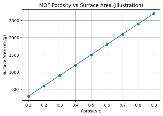

5. 交互式可视化（Interactive Visualization）¶

以下示例使用 Altair 创建简单的交互式可视化，展示 MOF 孔隙率与比表面积的关系。你可以通过刷选数据范围来高亮显示选中的数据点，并查看对应的统计信息。

import altair as alt
import numpy as np
import pandas as pd

# Generate MOF data with different types
np.random.seed(42)  # For reproducibility
mof_types = ['MOF-5', 'UiO-66', 'HKUST-1', 'MIL-101(Cr)', 'NU-1000']
phi_range = np.linspace(0.1, 0.9, 25)

# Create data for different MOF types with varying relationships
data_list = []
for mof in mof_types:
    # Different scaling factors for different MOFs
    if mof == 'MOF-5':
        scale_factor = 2.0
        base_sa = 1500
    elif mof == 'UiO-66':
        scale_factor = 1.8
        base_sa = 1200
    elif mof == 'HKUST-1':
        scale_factor = 2.2
        base_sa = 1800
    elif mof == 'MIL-101(Cr)':
        scale_factor = 2.5
        base_sa = 2000
    else:  # NU-1000
        scale_factor = 2.3
        base_sa = 1900
    
    for phi in phi_range:
        # Surface area relationship: varies by MOF type
        sa = base_sa + scale_factor * 5000 * phi
        
        data_list.append({
            'MOF_Type': mof,
            'Porosity': round(phi, 2),
            'Surface_Area': round(sa, 1)
        })

df = pd.DataFrame(data_list)

# Brush selection for interactive filtering
brush = alt.selection_interval(encodings=['x', 'y'])

# Main scatter plot with lines
points = alt.Chart(df).mark_point().encode(
    x=alt.X('Porosity:Q', 
            axis=alt.Axis(title='Porosity φ', format='.2f'),
            scale=alt.Scale(domain=[0.1, 0.9])),
    y=alt.Y('Surface_Area:Q', 
            axis=alt.Axis(title='Surface Area (m²/g)'),
            scale=alt.Scale(domain=[0, 15000])),
    color=alt.condition(brush, 'MOF_Type:N', alt.value('lightgray')),
    #size=alt.condition(brush, alt.value(80), alt.value(40)),
    tooltip=[
        alt.Tooltip('MOF_Type:N', title='MOF Type'),
        alt.Tooltip('Porosity:Q', title='Porosity', format='.2f'),
        alt.Tooltip('Surface_Area:Q', title='Surface Area', format='.1f')
    ]
).add_params(brush).properties(
    width=600,
    height=400,
    title='MOF Porosity vs Surface Area'
)

# Bar chart showing count of selected MOF types
bars = alt.Chart(df).mark_bar().encode(
    y=alt.Y('MOF_Type:N', axis=alt.Axis(title='MOF Type')),
    color='MOF_Type:N',
    x=alt.X('count():Q', axis=alt.Axis(title='Count'))
).transform_filter(brush).properties(
    width=600,
    height=200,
    title='Selected MOF Types Distribution'
)

# Combine charts vertically
points & bars

交互功能说明：

刷选区域：在主图表上拖拽鼠标选择数据范围，选中的数据点会高亮显示（有颜色），未选中的变为灰色
统计图表：下方的条形图会实时显示选中区域中各个 MOF 类型的数量分布
悬停提示：将鼠标悬停在数据点上可查看详细信息

6. Pandas 表格¶

import pandas as pd

df = pd.DataFrame({
    "MOF": ["MOF-5", "UiO-66", "HKUST-1"],
    "Metal": ["Zn²⁺", "Zr⁴⁺", "Cu²⁺"],
    "Surface Area (m²/g)": [3800, 1200, 1500]
})
df

7. 结构可视化（ASE）¶

（如果你的 kernel 安装了 ase）

7.1 ASE构造分子并交互显示¶

from ase.build import molecule
from ase.visualize import view

try:
    #Build a simple molecule with ASE
    water = molecule('H2O')
    
    #Visualize the molecule
    
    disp_water = view(water, viewer='x3d')
    display(disp_water)

except:
    print('ASE is not installed, so the example is skipped')

7.2 从本地文件读取结构并展示（CIF / POSCAR 等）¶

from ase.io import read

#Read structure from a local file, e.g. CIF\PDB
mof_from_file = read("../data/MOF-5.pdb")

#View the periodic structure
disp_mof=view(mof_from_file, viewer='x3d')
display(disp_mof)