MOF书籍示例第二章（进阶）

第二章：MOF 吸附与模拟¶

本章为MOF简介进阶章节，显示更多可以使用的功能和交互式代码

2.1 吸附等温线基础¶

MOF 在气体储存、分离等应用中，吸附等温线是非常重要的表征手段。

典型的 Langmuir 等温线可写为：

q(P) = q_{\max} \frac{b P}{1 + b P}

(1)

其中：

$q(P)$ ：在压力 $P$ 下的吸附量
$q_{\max}$ ：饱和吸附量
$b$ ：平衡常数（与温度有关）

2.2 MOF 吸附等温线可视化¶

不同的MOF拥有不同的吸附性能，比如第一章的1.2 典型结构示意与晶胞中示例的MOF结构。

下面示例展示不同 MOF 材料的吸附等温线特性。我们使用 Langmuir 模型来模拟典型的 MOF 吸附行为。

import numpy as np
import matplotlib.pyplot as plt

# Define Langmuir isotherm function
def langmuir_isotherm(P, qmax, b):
    """
    Langmuir isotherm model
    P: Pressure (bar)
    qmax: Saturation uptake (mmol/g)
    b: Equilibrium constant (bar^-1)
    """
    return qmax * b * P / (1 + b * P)

# Parameters for different MOFs (based on literature data)
mof_params = {
    'MOF-5': {'qmax': 8.5, 'b': 0.5, 'color': 'blue'},
    'UiO-66': {'qmax': 6.2, 'b': 0.8, 'color': 'green'},
    'HKUST-1': {'qmax': 7.8, 'b': 0.6, 'color': 'red'},
    'MIL-101(Cr)': {'qmax': 9.5, 'b': 0.4, 'color': 'orange'}
}

# Generate pressure range
P = np.linspace(0, 10, 200)

# Plot multiple isotherms
plt.figure(figsize=(10, 6))
for name, params in mof_params.items():
    q = langmuir_isotherm(P, params['qmax'], params['b'])
    plt.plot(P, q, label=name, color=params['color'], linewidth=2)

plt.xlabel("Pressure P (bar)", fontsize=12)
plt.ylabel("Uptake q (mmol/g)", fontsize=12)
plt.title("CO₂ Adsorption Isotherms for Different MOFs (Langmuir Model)", fontsize=14)
plt.legend(fontsize=10)
plt.grid(True, alpha=0.3)
plt.xlim(0, 10)
plt.ylim(0, 10)
plt.tight_layout()
plt.show()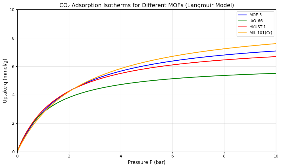

import numpy as np
import matplotlib.pyplot as plt

# Relationship between MOF porosity and surface area (empirical fit)
# Typical MOF porosity range: 0.3 - 0.9
phi = np.linspace(0.3, 0.9, 13)

# Empirical relation between surface area and porosity (simplified model)
# Most MOFs have specific surface area in the range 1000-7000 m²/g
surface_area = 2000 + 5000 * phi  # simplified linear relationship

# Representative MOF data points
mof_data = {
    'MOF-5': {'phi': 0.55, 'sa': 3800},
    'UiO-66': {'phi': 0.65, 'sa': 1187},
    'HKUST-1': {'phi': 0.68, 'sa': 1500},
    'MIL-101(Cr)': {'phi': 0.78, 'sa': 4230},
    'NU-1000': {'phi': 0.82, 'sa': 6143}
}

plt.figure(figsize=(8, 6))
plt.plot(phi, surface_area, 'b--', linewidth=2, label='Empirical Relation', alpha=0.7)

# Plot MOF data points
for name, data in mof_data.items():
    plt.scatter(data['phi'], data['sa'], s=100, alpha=0.7, 
                label=name, edgecolors='black', linewidth=1.5)

plt.xlabel("Porosity φ", fontsize=12)
plt.ylabel("Surface Area (m²/g)", fontsize=12)
plt.title("Relationship between MOF Porosity and Surface Area", fontsize=14)
plt.legend(fontsize=9, loc='upper left')
plt.grid(True, alpha=0.3)
plt.xlim(0.25, 0.95)
plt.ylim(0, 7000)
plt.tight_layout()
plt.show()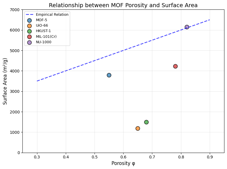

2.3 MOF 孔道中气体分子的扩散模拟¶

下面展示一个静态可视化示例，模拟气体分子在 MOF 孔道中的分布和扩散行为。我们使用随机游走模型来模拟分子在不同时间步的分布。

import numpy as np
import matplotlib.pyplot as plt
from matplotlib.patches import Rectangle

# Simulation parameters
np.random.seed(42)  # For reproducibility
n_particles = 50
n_steps = 100
box_size = 1.0

# Initialize: all molecules at center region
initial_positions = np.random.normal(0.5, 0.1, (n_particles, 2))
initial_positions = np.clip(initial_positions, 0.1, 0.9)

# Diffusion process (random walk)
positions = initial_positions.copy()
for step in range(n_steps):
    # Random step (related to diffusion coefficient)
    step_size = 0.02
    random_steps = np.random.normal(0, step_size, (n_particles, 2))
    positions += random_steps
    # Reflective boundary
    positions = np.clip(positions, 0.05, 0.95)

# Visualization
fig, axes = plt.subplots(1, 2, figsize=(14, 6))

# Left: initial distribution
ax1 = axes[0]
ax1.scatter(initial_positions[:, 0], initial_positions[:, 1], 
           c='blue', s=50, alpha=0.6, edgecolors='black', linewidth=0.5)
ax1.add_patch(Rectangle((0.1, 0.1), 0.8, 0.8, fill=False, 
                        edgecolor='gray', linewidth=2, linestyle='--'))
ax1.set_xlim(0, 1)
ax1.set_ylim(0, 1)
ax1.set_aspect('equal')
ax1.set_title("Initial: Molecules Clustered in Center Region", fontsize=12)
ax1.set_xlabel("Channel Position X", fontsize=10)
ax1.set_ylabel("Channel Position Y", fontsize=10)
ax1.grid(True, alpha=0.3)

# Right: after diffusion
ax2 = axes[1]
ax2.scatter(positions[:, 0], positions[:, 1], 
           c='red', s=50, alpha=0.6, edgecolors='black', linewidth=0.5)
ax2.add_patch(Rectangle((0.1, 0.1), 0.8, 0.8, fill=False, 
                        edgecolor='gray', linewidth=2, linestyle='--'))
ax2.set_xlim(0, 1)
ax2.set_ylim(0, 1)
ax2.set_aspect('equal')
ax2.set_title(f"After Diffusion ({n_steps} Steps): Molecules Evenly Spread", fontsize=12)
ax2.set_xlabel("Channel Position X", fontsize=10)
ax2.set_ylabel("Channel Position Y", fontsize=10)
ax2.grid(True, alpha=0.3)

plt.suptitle("Simulation of Gas Molecule Diffusion in MOF Channel", fontsize=14, y=1.02)
plt.tight_layout()
plt.show()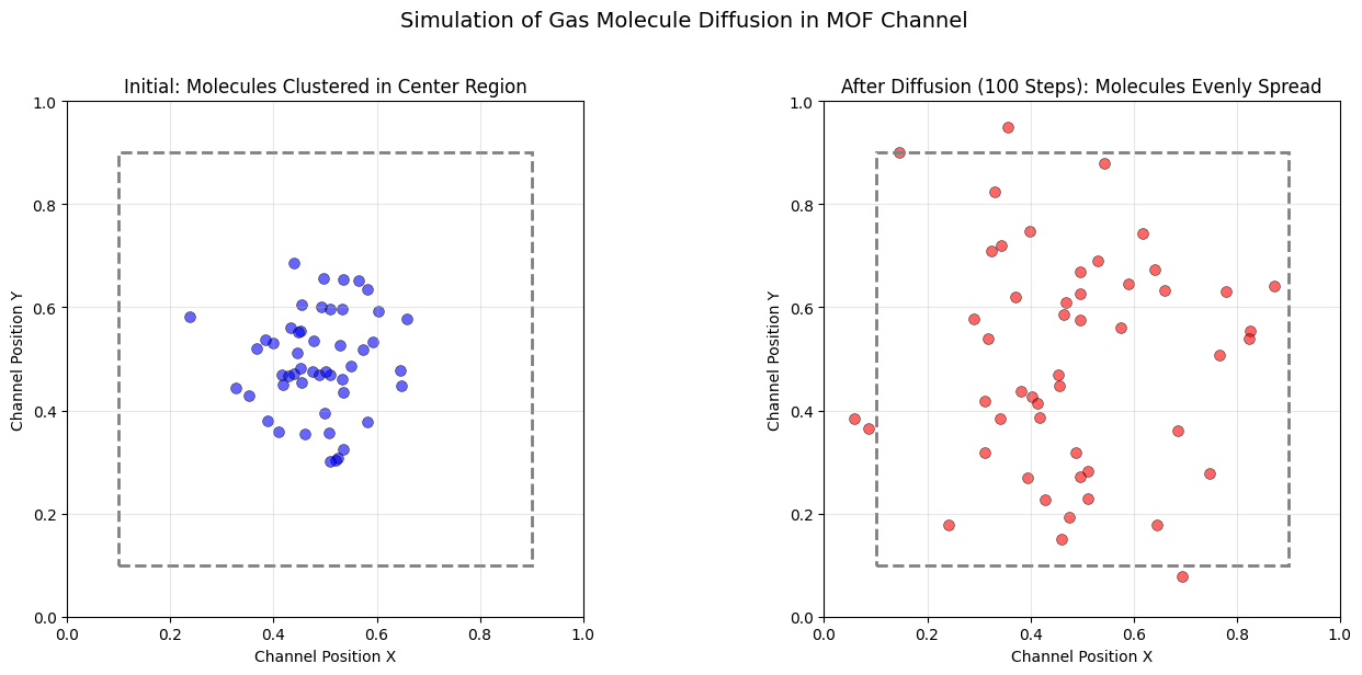

import numpy as np
import matplotlib.pyplot as plt

# Simulate molecular density distribution at different time steps
np.random.seed(42)
n_particles = 100
time_steps = [0, 20, 50, 100]
box_size = 1.0

fig, axes = plt.subplots(2, 2, figsize=(12, 12))
axes = axes.flatten()

initial_positions = np.random.normal(0.5, 0.1, (n_particles, 2))
initial_positions = np.clip(initial_positions, 0.1, 0.9)

for idx, n_steps in enumerate(time_steps):
    ax = axes[idx]
    positions = initial_positions.copy()
    
    for step in range(n_steps):
        step_size = 0.02
        random_steps = np.random.normal(0, step_size, (n_particles, 2))
        positions += random_steps
        positions = np.clip(positions, 0.05, 0.95)
    
    # Use 2D histogram to show density
    hist, xedges, yedges = np.histogram2d(positions[:, 0], positions[:, 1], 
                                          bins=20, range=[[0, 1], [0, 1]])
    extent = [0, 1, 0, 1]
    
    im = ax.imshow(hist.T, origin='lower', extent=extent, 
                   cmap='YlOrRd', interpolation='bilinear', aspect='equal')
    ax.add_patch(plt.Rectangle((0.1, 0.1), 0.8, 0.8, fill=False, 
                              edgecolor='black', linewidth=2))
    ax.set_title(f"Time Step t = {n_steps}", fontsize=11)
    ax.set_xlabel("Channel Position X", fontsize=9)
    ax.set_ylabel("Channel Position Y", fontsize=9)
    plt.colorbar(im, ax=ax, label='Molecule Density')

plt.suptitle("Time Evolution of Molecular Density in MOF Channel", fontsize=14, y=0.995)
plt.tight_layout()
plt.show()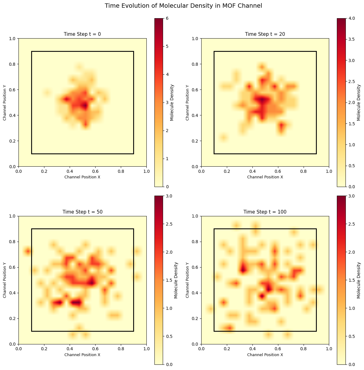

2.4 MOF 孔道中气体分子的行为定义¶

2.4.1 不同分子行为定义¶

吸附

解吸

扩散

吸附（adsorption）是气体或液体分子被「吸附到」固体表面或孔道中的过程。

2.4.2 模拟吸附过程简介¶

2.5 简易 GCMC 模拟¶

下面使用 Altair 实现一个可交互的 GCMC（大正则蒙特卡洛）模拟 MOF 吸附过程的可视化。你可以拖动化学势 $\mu$ 的滑块，实时观察气体分子数均值的演化与分布。

import altair as alt
import numpy as np
import pandas as pd

# Simplified GCMC algorithm
def gcmc_sim(mu=-1.5, beta=1.0, V=100.0, n_steps=1000, seed=42):
    np.random.seed(seed)
    N = 0
    N_list = []
    for step in range(n_steps):
        if np.random.rand() < 0.5:
            # Insert
            dE = 0.5 * N
            acc = min(1, np.exp(-beta * dE + beta * mu + np.log(V/(N+1))))
            if np.random.rand() < acc:
                N += 1
        else:
            # Remove
            if N > 0:
                dE = 0.5 * (N-1)
                acc = min(1, np.exp(-beta*(-dE) - beta*mu + np.log(N/V)))
                if np.random.rand() < acc:
                    N -= 1
        N_list.append(N)
    return N_list

# Generate GCMC statistics for different μ values
# Use ALL mu values that are multiples of 0.05 to match slider step exactly
# This ensures slider can match ALL possible values (2.75, 2.8, 2.85, etc.)
mu_list = np.arange(-3.0, 0.05, 0.05)  # -3.0, -2.95, -2.9, -2.85, ..., -0.05 (60 values)
# All values are multiples of 0.05, matching slider step perfectly
steps = 300  # Reduced steps to keep total data size manageable
results = []

for mu in mu_list:
    # Round to 2 decimal places to avoid floating point precision issues
    mu_rounded = np.round(mu, 2)
    N_hist = gcmc_sim(mu=mu_rounded, n_steps=steps)
    # Downsample: take every 4th point to reduce data size (60 mu * 75 points = 4500 rows)
    for i in range(0, len(N_hist), 4):
        results.append({
            'mu': mu_rounded,  # Use the rounded value
            'Step': i,
            'N': N_hist[i]
        })

df = pd.DataFrame(results)

# Mean adsorption statistics
df_mean = df.groupby('mu').agg(meanN=('N','mean'), stdN=('N','std')).reset_index()

# Altair slider using param (Altair v5+)
slider = alt.binding_range(min=-3, max=0, step=0.05, name='μ (chemical potential)=')
mu_select = alt.param(
    bind=slider,
    value=-1.5
)

# 1. Evolution curve (top panel, full width)
# Now mu values are exact multiples of 0.05, use small tolerance for matching
line_evo = alt.Chart(df).mark_line(opacity=0.7, strokeWidth=2).encode(
    x=alt.X('Step:Q', axis=alt.Axis(title='MC Step')),
    y=alt.Y('N:Q', axis=alt.Axis(title='Number of molecules (N)')),
    color=alt.Color('mu:O', legend=None),
    tooltip=['Step', 'N', 'mu']
).transform_filter(
    # Use small tolerance (0.01) since data mu values are multiples of 0.05
    # This will match when slider is within 0.01 of a data point
    (alt.datum.mu >= mu_select - 0.01) & (alt.datum.mu <= mu_select + 0.01)
).properties(
    width=800, height=250,
    title='GCMC Simulation: Evolution of N vs. MC Step'
).add_params(mu_select)

# 2. Adsorption isotherm
ads_iso = alt.Chart(df_mean).mark_line(interpolate='monotone', point=True).encode(
    x=alt.X('mu:Q', axis=alt.Axis(title='Chemical potential μ', format='.2f')),
    y=alt.Y('meanN:Q', axis=alt.Axis(title='Mean adsorbed molecules ⟨N⟩')),
    tooltip=['mu','meanN','stdN'],
    color=alt.value('#1367a7')
).properties(
    width=400, height=250,
    title='MOF Adsorption Isotherm (GCMC Simulation)'
)

selected = ads_iso.mark_point(size=120, filled=True, color='crimson').encode(
    x='mu:Q', y='meanN:Q'
).transform_filter(
    (alt.datum.mu >= mu_select - 0.01) & (alt.datum.mu <= mu_select + 0.01)
)

# 3. Histogram of N
hist = alt.Chart(df).mark_bar(color='#E09842').encode(
    x=alt.X('N:Q', bin=alt.Bin(maxbins=30), title='Number of molecules N'),
    y=alt.Y('count():Q', title='Count'),
    tooltip=['N','count()']
).transform_filter(
    (alt.datum.mu >= mu_select - 0.01) & (alt.datum.mu <= mu_select + 0.01)
).properties(
    width=400, height=250,
    title='Distribution of N during MC'
)

# Combine panels: Evolution on top, Histogram and Isotherm side by side below
panels = (
    line_evo & (hist | (ads_iso + selected))
).resolve_scale(y='independent')

# Display the chart
panels

你可以拖动「 $\mu$ （化学势）」滑块，在不同 $\mu$ （代表不同气体压力/浓度）下动态地观察：

气体分子数随 MC 步数的变化趋势
吸附均值 $\langle N \rangle$ 随 $\mu$ 的变化（吸附等温线）
MC 过程中 $N$ 的分布直方图

本交互式可视化便于科研人员或学生直观理解和探索 MOF 吸附过程以及 GCMC 思路。