Author Template - 2. Code - Authoring Guide

Abstract¶

Contains examples of all MyST markdown code syntax

Code Section¶

This chapter demonstrates advanced usage of {code-cell}.
All the examples are themed around MOF structure modeling / adsorption simulation / materials property calculation.

1. Static Code (Not Executed)¶

Block content:

:::{code} python
def mof_density(M, V):
    return M / V
print(mof_density(1000, 500))
:::

def mof_density(M, V):
    return M / V
print(mof_density(1000, 500))

Suitable for: Concept explanations / example code snippets

2. Executable code-cell¶

(Requires kernelspec at the top of the file and running myst start --execute)

:::{code-cell} python
import numpy as np
print("Example: generate random porosity:", np.random.rand())
:::

import numpy as np
print("Example: generate random porosity:", np.random.rand())

Example: generate random porosity: 0.8708862896410129

3. Add Metadata¶

Metadata can control the way code is executed and displayed.

3.1 Hide Input (only show output)¶

Block content:

:::{code-cell} python
:tags: hide-input
print('MOF is great')
:::

MOF is great

3.2 Hide Output (only show code)¶

Block content:

:::{code-cell} python
:tags: hide-output

x = 42
x
:::

x = 42
x

3.3 Completely Remove Input (code is invisible in the final webpage)¶

Block content:
:::{code-cell} python
:tags: remove-input

print("This code is not visible in the final webpage, but still executed")
:::

print("This code is not visible in the final webpage, but still executed")

This code is not visible in the final webpage, but still executed

3.4 Completely Remove Output (output not visible on webpage)¶

Block content:

:::{code-cell} python
:tags: remove-output

print("This code is not visible in the final webpage, but still executed")

print("This code is not visible in the final webpage, but still executed")

Frequently Used Tags¶

tag	Meaning
hide-input	Hide code, show output only
hide-output	Hide output
remove-input	Completely remove input on the page
remove-output	Completely remove output
raises	Specify expected exceptions
cache	Allow execution caching

4. Plotting¶

The following example shows a plot of the relationship between MOF porosity and surface area.

import numpy as np
import matplotlib.pyplot as plt

phi = np.linspace(0.1, 0.9, 9)
sa = 1500 * phi * 2

plt.figure(figsize=(6,4))
plt.plot(phi, sa, marker="o")
plt.xlabel("Porosity φ")
plt.ylabel("Surface Area (m²/g)")
plt.title("MOF Porosity vs Surface Area (illustration)")
plt.grid(True)
plt.show()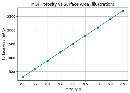

5. Interactive Visualization¶

The following example uses Altair to create a simple interactive visualization of MOF porosity and surface area. You can brush-select a data range to highlight selected points and view corresponding statistics.

import altair as alt
import numpy as np
import pandas as pd

# Generate MOF data with different types
np.random.seed(42)  # For reproducibility
mof_types = ['MOF-5', 'UiO-66', 'HKUST-1', 'MIL-101(Cr)', 'NU-1000']
phi_range = np.linspace(0.1, 0.9, 25)

# Create data for different MOF types with varying relationships
data_list = []
for mof in mof_types:
    # Different scaling factors for different MOFs
    if mof == 'MOF-5':
        scale_factor = 2.0
        base_sa = 1500
    elif mof == 'UiO-66':
        scale_factor = 1.8
        base_sa = 1200
    elif mof == 'HKUST-1':
        scale_factor = 2.2
        base_sa = 1800
    elif mof == 'MIL-101(Cr)':
        scale_factor = 2.5
        base_sa = 2000
    else:  # NU-1000
        scale_factor = 2.3
        base_sa = 1900
    
    for phi in phi_range:
        # Surface area relationship: varies by MOF type
        sa = base_sa + scale_factor * 5000 * phi
        
        data_list.append({
            'MOF_Type': mof,
            'Porosity': round(phi, 2),
            'Surface_Area': round(sa, 1)
        })

df = pd.DataFrame(data_list)

# Brush selection for interactive filtering
brush = alt.selection_interval(encodings=['x', 'y'])

# Main scatter plot with lines
points = alt.Chart(df).mark_point().encode(
    x=alt.X('Porosity:Q', 
            axis=alt.Axis(title='Porosity φ', format='.2f'),
            scale=alt.Scale(domain=[0.1, 0.9])),
    y=alt.Y('Surface_Area:Q', 
            axis=alt.Axis(title='Surface Area (m²/g)'),
            scale=alt.Scale(domain=[0, 15000])),
    color=alt.condition(brush, 'MOF_Type:N', alt.value('lightgray')),
    #size=alt.condition(brush, alt.value(80), alt.value(40)),
    tooltip=[
        alt.Tooltip('MOF_Type:N', title='MOF Type'),
        alt.Tooltip('Porosity:Q', title='Porosity', format='.2f'),
        alt.Tooltip('Surface_Area:Q', title='Surface Area', format='.1f')
    ]
).add_params(brush).properties(
    width=600,
    height=400,
    title='MOF Porosity vs Surface Area'
)

# Bar chart showing count of selected MOF types
bars = alt.Chart(df).mark_bar().encode(
    y=alt.Y('MOF_Type:N', axis=alt.Axis(title='MOF Type')),
    color='MOF_Type:N',
    x=alt.X('count():Q', axis=alt.Axis(title='Count'))
).transform_filter(brush).properties(
    width=600,
    height=200,
    title='Selected MOF Types Distribution'
)

# Combine charts vertically
points & bars

Interactive Functionality Instructions:

Brushing Selection: Drag the mouse on the main chart to select a data region; selected points will be highlighted (in color), unselected will be gray
Statistics Chart: The bar chart below will show the count distribution of each MOF type in the selected region in real time
Tooltip: Hover over any data point to see details

6. Pandas Table¶

import pandas as pd

df = pd.DataFrame({
    "MOF": ["MOF-5", "UiO-66", "HKUST-1"],
    "Metal": ["Zn²⁺", "Zr⁴⁺", "Cu²⁺"],
    "Surface Area (m²/g)": [3800, 1200, 1500]
})
df

7. Structure Visualization (ASE)¶

(If your kernel has ase installed)

7.1 Build molecule via ASE and show interactively¶

from ase.build import molecule
from ase.visualize import view

try:
    # Build a simple molecule with ASE
    water = molecule('H2O')
    
    # Visualize the molecule
    disp_water = view(water, viewer='x3d')
    display(disp_water)

except:
    print('ASE is not installed, so the example is skipped')

7.2 Read and show structure from local file (CIF / POSCAR etc.)¶

from ase.io import read

# Read structure from a local file, e.g. CIF/PDB
mof_from_file = read("../data/MOF-5.pdb")

# View the periodic structure
disp_mof=view(mof_from_file, viewer='x3d')
display(disp_mof)